Chapter 2 The ATLAS Experiment

The ATLAS detector is a general-purpose experiment, designed to explore physics phenomena on a wide energy scale, ranging from 100 GeV --- the lower limit for the mass of the Higgs boson --- up to 1 TeV and beyond --- where SUSY or exotic physics could hide. In order to fully exploit the opportunities given by the LHC collider, ATLAS needs to be versatile enough to sustain the challenges presented by the experimental environment; in order to accomplish this goal, the instrumentation of the ATLAS detector includes:

a vertex detector for the measurement of the impact parameters of the primary interaction vertex and for the identification of secondary vertices coming from the decay of short-lived particles (b,t);
high-precision trackers for the accurate measurement of momenta of charged particles in a high-occupancy environment;
hadronic and electromagnetic calorimeters for the identification of electrons, pions, photons and hadronic jets and for the measurement of E_T^miss;
a muon spectrometer for the stand-alone measurement of high-p_T muons.

The configuration of the ATLAS detector is typical for experiments at particle colliders: ATLAS is a symmetric cylinder 40 m long and with a diameter of 22 m. The instrumentation of the detector is arranged in concentric layers around the beam axis (the barrel section) and in two wheels (the end-caps) located at the extremities of the cylinder.

The first barrel layer, located next to the interaction point, is the Inner Detector; this apparatus is composed of three sub-detectors: (from inside to outside) the Pixel Detector, the Semi-Conductor Tracker and the Transition Radiation Tracker. The task of the Inner Detector is the reconstruction of primary and secondary vertices and the measurement of momenta of charged particles. The reconstruction of secondary vertices is crucial for the identification of b-quarks (see Section 1.7.1).

Outside the Inner Detector is located a cryostat which contains the Central Solenoid and the Liquid Argon calorimeter. The Central Solenoid is a superconducting coil generating a 2 T solenoidal magnetic field, oriented along the beam axis, which provides the lever arm to measure the particles' momenta in the Inner Detector. The Liquid Argon calorimeter is responsible for the measurement of the energy of electromagnetic showers (electrons, photons). The ATLAS calorimetry is completed by the TileCal calorimeter, which measures the energy of hadronic jets and acts as a yoke for the return flux of the solenoidal magnetic field.

The outermost ATLAS barrel layer is the Muon Spectrometer. The spectrometer uses a separate magnetic field, generated by eight superconducting coils deployed radially around the beam axis; the peculiar positioning of the coils creates a 4 T toroidal magnetic field that encompasses the whole spectrometer.

The two end-caps are identical and are composed of a cryostat containing the Liquid Argon electromagnetic and hadronic calorimeters. Behind the cryostat is located a wheel of Cathode Strip Chambers, which are part of the Muon Spectrometer. The end-caps have their own 4 T toroidal magnetic fields, which are generated by two eight-coil toroids encased in two cryostats which plug in the ATLAS barrel. The end-cap wheels of the Muon Spectrometer are placed between the ATLAS end-caps and the wall of the underground experimental area. The ATLAS detector is completed by two high-density Forward Calorimeters which guarantee the hermeticity of the detector at high rapidities. Two beam shields connect ATLAS to the LHC accelerator and protect the end-cap instrumentation from beam radiation and RF waves.

2.1 The Combined Test Beam setup

The components of the ATLAS detector have been tested at CERN for several years. The tests used a proton beam from the SPS accelerator, which was divided in several branches and sent to different test areas. In the test areas, the proton beam collided with a target to produce secondary particles such as electrons and pions; the secondary particles were collected, focused, and sent to the detectors being tested. The secondary particles could also be sent on another target, in order to produce a tertiary muon beam. The particle beams were monochromatic, with energies varying from 1 to 350 GeV.

Anno 2004 marked the last year of test beams at CERN; from 2005 the SPS will be subjected to upgrades that will finally result in this glorious accelerator being integrated in LHC's complex machinery. The last year of tests was dedicated to the Combined Test Beam (CTB): the test layout was designed to simulate a slice of the barrel of the ATLAS detector, with all the sub-detectors tested and read out at the same time, and with the trigger and data flow architectures as much close as the final design as possible. The software used to reconstruct the physics data was also standard ATLAS software.

The layout of the ATLAS slice is shown in Figure 2.1: in the first stage of the setup, a "cold box" containing Pixel and SCT modules was mounted inside a 0.4 Tm magnet, bending particle tracks in the horizontal plane. Behind the cold box, six TRT modules were placed, to complete the Inner Detector mock up.

Downstream from the Inner Detector, the Calorimetry layout was composed of a cryostat, containing the LAr module 0, and three TileCal modules. The calorimeter setup was placed on a rotating and tilting frame, which allowed to evaluate the performance of calorimetry at various h and f positions.

The mock-up of the Muon Spectrometer included both chambers from the barrel and the end-cap sectors. The barrel sector comprised a full projective tower, with six barrel MDT chambers and six RPC chambers; and the end-cap sector contained a full wheel sector with six end-cap MDT chambers, two TGC doublets and one TGC triplet. Given the impossibility of deploying a magnetic field on a scale of several metres, the "point and angle" measurement technique was implemented (see Section 1.7.6). One extra MDT-RPC station was placed in front of a 2 Tm magnet, while the rest of the spectrometer instrumentation was placed behind the magnet. The muon momentum was measured by computing the deflection of the muon tracks before and after the magnet.

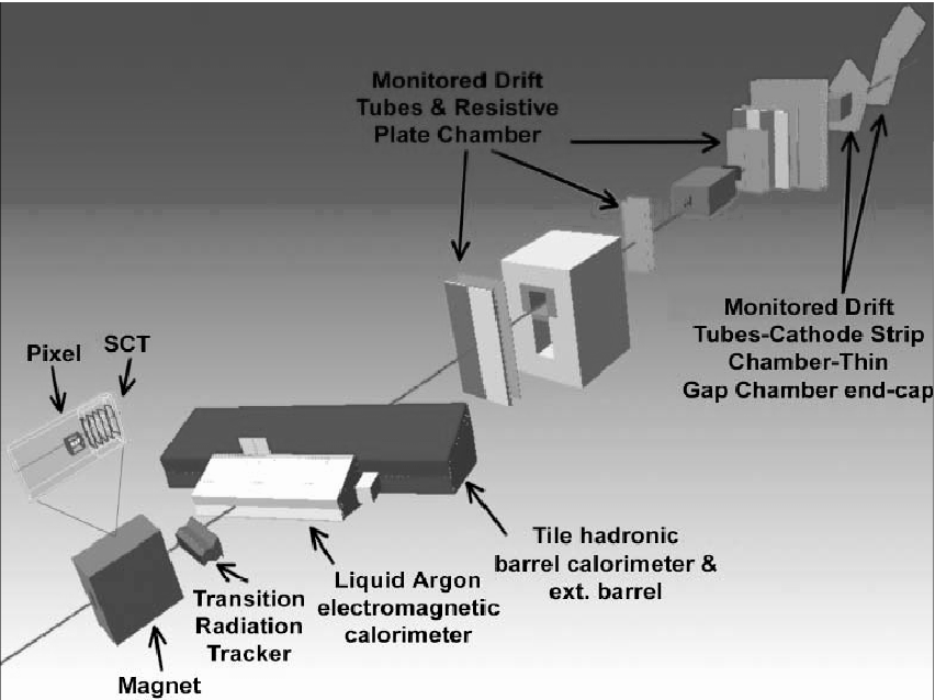
Figure 2.1: Layout of the Combined Test Beam 2004. From left to right: The "cold box" containing the Pixel and SCT modules, embedded in the bending magnet; the TRT modules; the LAr and TileCal calorimeter modules mounted on a rotating frame (not shown); the Muon Spectrometer setup including a bending magnet, six MDT barrel chambers and six MDT end-cap chambers. The trigger RPC and TGC chambers are mounted on the MDT chambers. One extra MDT-RPC station is placed before the spectrometer magnet to evaluate the track deflection. The unmarked blocks in the spectrometer indicate passive material used to mock the magnet coils and support structures of the spectrometer.

2.2 The Inner Detector

The Inner Detector is the innermost instrument of the ATLAS experiment. The goals of this detector are:

identify the primary interaction vertex and measure the impact parameter with a resolution s_d=11+60/p_Tsinq µm and s_z=70+100/p_Tsin³q µm [28];
identify secondary vertices (for b-tagging);
measure p_T of charged particles with a resolution of 30% at p_T=500 GeV, with a pseudorapidity coverage of |h|<2.5¹.

The Inner Detector is composed of three sub-detectors: two of them (the Pixel Detector and the Semi Conductor Tracker) are based on reverse-biased semiconductor technology, while the third one (the Transition Radiation Tracker) is a gaseous detector. The use of different technologies is the result of a trade-off between high spatial resolution and a lightweight detector. Semiconductor detectors guarantee a high precision in the measurement of space points and tracks --- typically the resolution is of the same order magnitude of the size of the active elements of the detector, that is tens of microns. The density of the semiconductor substrate and the need for bulky cooling and readout services implies high interaction and radiation lengths, which can cause multiple scattering and energy loss of the incoming particle, resulting in a degradation of the quality of measurements for the detectors which are downstream of the Inner Detector. The choice of ATLAS was to limit the amount of semiconductor by including in the Inner Detector a gaseous tracker, which is more "transparent" to incoming particles, can measure a higher number of space points along the particles' tracks without multiple scattering and can exploit the transition radiation phenomenon to identify electrons and charged pions.

2.2.1 The Pixel Detector

The pixel detector is composed of three cylindrical barrel layers and five wheels on each side of the barrel. The barrel layers are located at 50.5, 88.5 and 122.5 mm from the beam axis. The intermediate layer will not be included in the initial ATLAS layout and will be installed at a later stage. The effect of staging on b-tagging and secondary vertex reconstruction has been summarised in Section 1.7.1.

The barrel layers are made of identical staves; each stave is composed of 13 pixel modules, inclined 20 with respect to the cylinder's tangent. The inclination of the modules is designed to counterbalance the effect of the magnetic field on charged particles, keeping the particle's tracks as orthogonal as possible to the pixel modules. The pixel wheels are organised in sectors, and use the same module type as the barrel staves.

The pixel module is made of a silicon wafer, divided in 16 units. Each of the units is composed of columns and rows of pixels of sizes 50400 µm--- the pixel dimension has been increased with respect to the TDR nominal size, with effects on the vertex identification (see Section 1.7.1). Each pixel is a reverse-biased p-n junction, and it is bump-bonded to a front-end (FE) readout chip. In a pixel modules there are 16 front-end chips, one for each pixel unit of the module. The front-end chip contains one pre-amplifier and a fast discriminator for each pixel channel. The signal from the pixels is passed through the discriminator, and if the height of the signal is above the discriminator threshold, a hit is registered for the firing pixel, and a timestamp for the leading and trailing edge of the above threshold pulse is digitized in a 25-bit data word, together with the pixel location [31]. The front-end chip contains an End-of-Column (EoC) circuit which reads the digital data out the pre-amp/discriminator stages of all pixels and sends the data to the Module Control Chip (MCC). There is one MCC per pixel module, which has the task of collecting data from the 16 front-end chips, providing power to the pixels and enabling/disabling individual pixels. The MCC is powered by a Kapton²/flex hybrid support and sends data to higher levels of the Data Acquisition system by optical links. The module cross-section is shown in Figure 2.2. Since the front-end chips are smaller than the wafer area, there is a 200 µm gap of potentially uninstrumented pixels between adjacent chips. To remedy this fact, pixels between FE chips are longer (50600 µm) and share readout channels; as a result, 5% of the pixel channels have a two-fold ambiguity that will be resolved off-line [33].

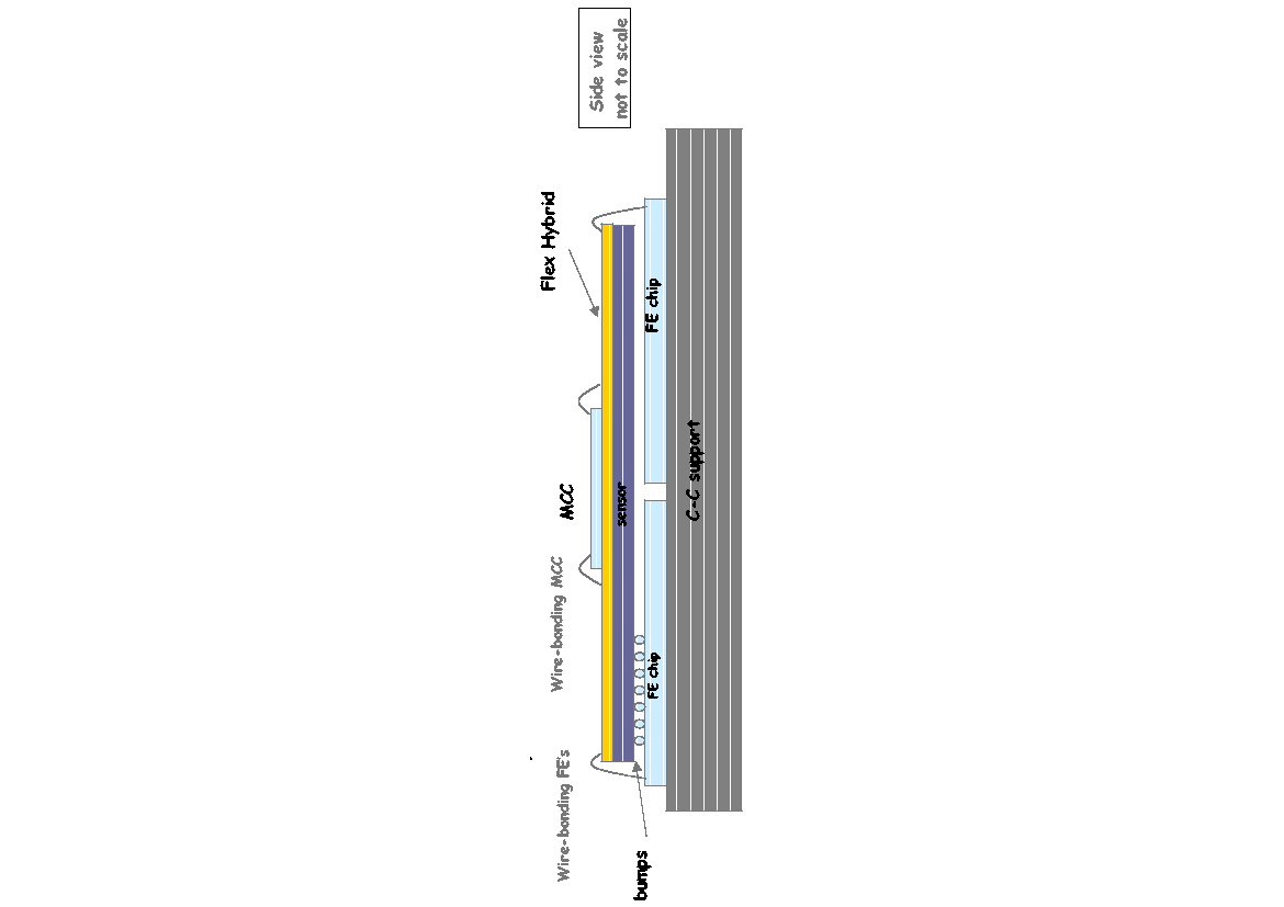
Figure 2.2: Cross-section of a pixel module. The MCC and the wafer sensor are glued onto a Kapton/flex hybrid which provides power to the module. The MCC delivers power to the sensor and the Front-End chips via wire bonding. Signal from the sensor is transmitted to the FE chips via bump-bonds. The figure shows also the carbon structure which gives mechanical stability to the module. Note the 200 µm gap between the FE chips (see text). Figure taken from [34].

2.2.2 The Semi Conductor Tracker

The Semi Conductor Tracker is composed of 4 concentric cylindrical layers placed on radii ranging from 30 to 52 cm away from the beam axis. On both sides of the barrel layers, 9 wheels are placed to extend the coverage of the SCT up to |h|<2.5. The barrel layers are made of "ladders" covering the whole f range; each ladder is made of 12 detector modules. The detector modules are made of 4 wafers: each wafer is composed of 768 semiconductor strips, 63.6 mm long with a pitch of 80 µm; each strip is capacitively coupled to an aluminium strip which is used for signal readout. The detector modules are divided in a front side and a back side: on the front side, two strip units are bump bonded together, creating a single array of strips twice the length of the initial strip unit. The back side is built in the same way, and it is rotated of 40 mrad with respect to the front side. The small stereoscopic angle is used to track impinging particles in the z coordinate; a small angle is preferred to an orthogonal arrangement of strips because it reduces the impact of ghost hits in pattern recognition for high-multiplicity events. Detector modules for the SCT wheels are built in a similar way, the only difference being that wheel modules are tapered in order to be arranged in circular sectors. The barrel modules are mounted at 10 with respect to the barrel tangent to reduce the effect of the magnetic field on the tracks of charged particles.

Both sides of the detector module are read out by individual hybrid chips, which are composed of a pre-amplifier/shaper/discriminator stage --- one circuit for each strip --- and a pipeline that stores hits until a request for data arrives from the trigger. The data is stored in binary format and it consists only of those strips whose signal exceeded the discriminator threshold; the data does not contain information neither about the height of the signal peak nor the time above threshold.

2.2.3 The Transition Radiation Tracker

The Transition Radiation Tracker TRT is the outermost component of the Inner Detector of the ATLAS experiment. Its novel design combines the tracking capabilities of a drift tube chamber with the electron/pion rejection of a transition radiation detector.

The TRT is composed by 370000 carbon fibre drift tubes with an inner conductive Kapton layer --- which are called straws; each straw is 4 mm in diameter and contains a 30 µm gold-plated anode wire. The straws are embedded in polypropylene foils or fibres --- which act as radiators --- and filled with a gas mixture of 70% Xenon, 27% Carbon Dioxide and 3% Oxygen [38]. Each anode wire is read out by the TRT front-end electronics, which is composed by an amplifier-shaper-discriminator chip (ASDBLR) and a time digitizer (DTMROC).

The TRT straws have a dual function: they can perform particle track measurements and they can detect transition radiation (see Section 1.7.5). When a charged particle crosses the detector, it will on average cross 35 straws, generating a low threshold signal --- typically 200 eV --- in each straw. The drift time of each individual straw can be measured and, calculating the radius of closest approach of the particle to the anode wire, the track of the particle can be fitted. Each straw has a spatial resolution of 170 µm and the TRT can measure the momentum of charged particles down to p_T~0.5 GeV. At the same time, as the particle crosses the polypropylene fibres, a virtual oscillating dipole forms between the particle and the polypropylene, resulting in the emission of transition radiation (X-rays) along the particle track. The Xenon contained in the straws has a high absorption, thus the X-rays generate a high threshold signal on the anode wire --- corresponding to an energy deposition of several keV. The ASDBLR chip amplifies the signal, shapes it and discriminates the signal against the two thresholds. The discriminated signal is passed to the DTMROC, which digitizes the pulse in 3.125 ns time bins. The data output from the DTMROC contains the status of the low threshold signal over three consecutive bunch crossings and the status of the high threshold signal.

The TRT is built from three components: a barrel and two end-caps. In the TRT barrel, three concentric layers of 32 modules are located outside of the SCT detector, in the region 56 <r< 107 cm and |z|< 72 cm, corresponding to a pseudorapidity coverage of |h|< 0.7; the straws are 144 cm long and run parallel to the beam axis. The straws are embedded in a matrix of polypropylene fibres and the anode wires are electrically split in the middle of the straws and read out on both sides, in order to reduce the occupancy.

The end-cap modules are both composed of 18 circular modules called wheels. In each wheel, layers of radial straws are interleaved with polypropylene foils; the straws occupy a radius between 63 and 103 cm around the beam axis. The installation of the last four wheels --- that in the original design would have occupied a radius between 47 and 100 cm, covering a pseudorapidity range of 1.7 <|h|< 2.5 --- has been postponed to the high luminosity phase.

Tracking performance

At the time of writing, the combined performance of the tracking efficiency of the TRT with the Pixel Detector and the Semiconductor Tracker has not been estimated yet.

Particle identification performance

Particle identification (e/p, e/µ) has been performed at the H8 test-beam in 2004. The test was designed to estimate the electron efficiency and the pion rejection factor and to compare the test-beam values with the values quoted in the TDR. The beam was composed of a mixture of muons, pions and electrons with energies ranging from 1 to 180 GeV. In order to be able to estimate the efficiency of the TRT, an independent system of identification needed to be set up; shower shapes from the electromagnetic calorimeter and measurements of the boost of the particle from a dedicated Cerenkov detector were used at H8.

Each track of the TRT was extrapolated to the calorimeter and matched with a cell cluster. The shape of the cluster was used as one of the discriminating factors: the electromagnetic calorimeter is segmented in three sampling regions plus a pre-shower (see Section 2.3.1), and the electrons tend to deposit most of their energies in the second sampling region of the calorimeter. Then, defining EMFn as the ratio between the energy deposited in the n-th sampling region of the calorimeter and the nominal beam energy (EMF0 indicates the pre-shower), and combining this variables with the γ (boost) measurements of the Cerenkov detector, the following selection cuts are defined for high energy (100 GeV) beams [42]:

electrons: γ>1000, EMF1>0.1, EMF2>0.2;
pions: γ<600, 0.02<EMF1<0.4, 0.02<EMF2<0.5;
muons: γ<600, EMF1<0.02, EMF2<0.02;

while for low energy beams (2-9 GeV) a different set of cuts is used, which takes into account the ration (LArF) between the total energy measured in the LAr and the nominal beam energy (different LArF cuts were put in place for beams of respectively 2,3,5 and 9 GeV) [43]:

electrons: γ>700, EMF0<0.1, EMF1+EMF2>0.05, EMF1>0.2, LArF>0.7-0.8;
pions: γ<600, EMF0<0.1, EMF1+EMF2>0.05, EMF1<0.1, LArF>0.4-0.7;
muons: EMF1+EMF2<0.05.

Once a track has been matched with a particle type, the number of high threshold straw hits along the track is counted. Since the number of high threshold hits along a track is higher for electron tracks than for pion tracks (see Figure 2.3), the pions can be rejected by a suitable cut on hit multiplicity (see Figure 2.4).

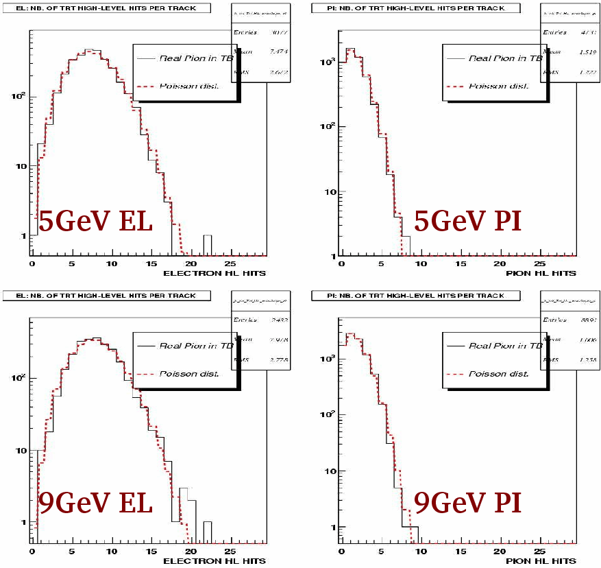
Figure 2.3: High threshold hit multiplicities for electrons (left) and pions (right) of 5 and 9 GeV. The continuous line plots test beam data, while the dashed line plots a Montecarlo simulation, assuming a Poisson distribution for hit multiplicities. Figure taken from [43].

The rejection factor for pions can be plotted against the electron efficiency, and the working point of the TRT can be selected by choosing an acceptable trade-off between the electron efficiency and the pion rejection factor. The difference in high threshold hit multiplicities in the TRT straws remains almost constant for a range of energies from 2 to 9 GeV, allowing for cuts with a high pion rejection on this energy range (see Figure 2.4). Figure 2.5 shows the comparison between the rejection/efficiency curve obtained by applying the cuts on test beam data and the optimal curve described in the ATLAS TDR.

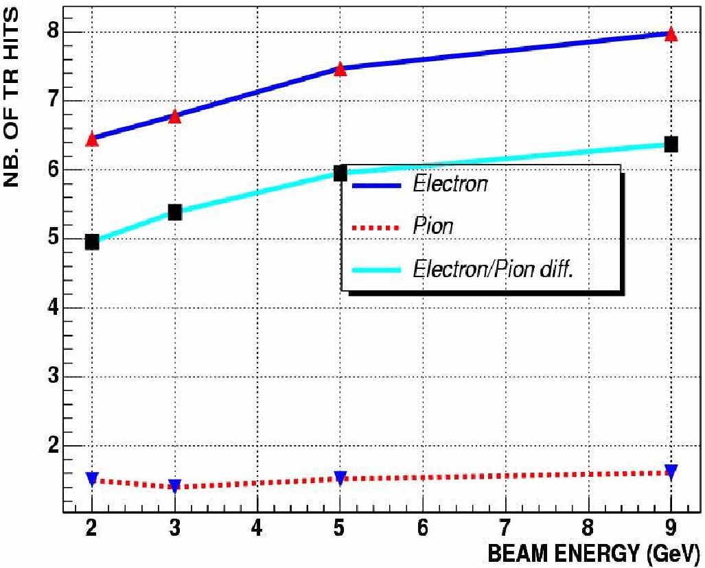
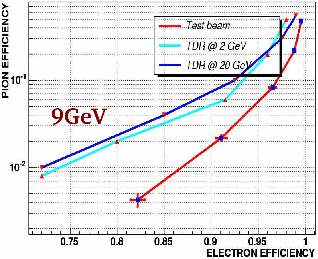
Figure 2.4: High threshold hit multiplicities in the TRT straws for electrons and pions, with energies varying from 2 to 9 GeV. The difference in hit multiplicity for electrons and pions is almost constant on the given energy range, allowing to introduce a reliable cut on the high threshold hits. Figure taken from [43].

Figure 2.5: Rejection/efficiency plots for electron/pions at the test beam and the nominal TDR performance. Test-beam data includes 9 GeV electrons and pions, while the TDR plots refer to the same particles with an energy of 2 and 20 GeV. Figure taken from [43].

2.2.4 Combined test results

The tracking resolution of the Inner Detector was tested in 2004. The setup consisted of 3 pixel layers, of 2 modules each, simulating two pixel staves of the ATLAS detector. The two staves were overlapping for a length of 1 mm. The SCT sector simulated four barrel layer of two modules each, with an overlap of 3 mm. The pixel and SCT modules were situated in a "cold box" which kept the modules at a temperature of 0 C. The cold box was located inside a magnet, which exposed the modules to a magnetic field that could be set from 0 to 1.4 Tesla; the magnetic field was directed horizontally and perpendicular to the particle beam. In front of the magnet were placed six TRT modules for a total of 3284 straws, simulating 1/16th of the ATLAS TRT barrel. At the time of writing, the TRT data was not included in the tracking performance of the Inner Detector because of difficulties in the calibration of the TRT modules.

The alignment procedure proceeds as follows: first of all, tracks are reconstructed in the stand-alone Pixel detector: the reconstruction algorithm selects only those tracks which cross the overlap between modules; the tracks are fitted by minimizing 5 parameters (y₀,z₀,f,q,y) which describe the relative positions of the modules; this way, it is possible to align internally all the modules of the Pixel detector. The same internal alignment procedure is applied to the SCT modules. Once the Pixel and SCT are internally aligned --- with a resolution of, respectively 12 and 25 µm [37] --- the SCT tracks are extrapolated back to the Pixel detector, obtaining the parameters for the relative alignment of the SCT with the respect of the Pixel detector. When all the parameters have been determined, global tracks can be fitted through both detectors. The procedure was tested for electron beams of 5 and 9 GeV, and the fitting of helices allowed the measurement of electron energies (see Figure 2.6).

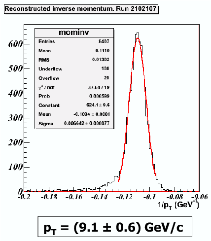
Figure 2.6: Inverse momentum resolution for combined Pixel/SCT electron tracks. Figure taken from [37].

2.3 Calorimetry

The calorimetry system of the ATLAS detector is based on two different technologies: the Liquid Argon (LAr) technology and the scintillating tile technology. Liquid Argon detectors measure the ionisation charge created in a volume of Argon by incoming particles; the ionisation charge drifts in the electric field gnerated by high voltage electrodes and it is finally collected by readout electrodes. Since for showering particles the ionisation charge is, on average, proportional to the energy of the incoming particle, the measured charge gives an estimate of the energy of the particle. In order to increase the ionisation charge, the Argon density is increased by cooling the gas down to the liquid phase; all LAr detectors need cryostats and cooling services, that can induce incoming particles to scatter and lose energy outside the detector volume, degrading the energy resolution. In order to contain the particle inside the calorimeter and enhance energy deposition in the fiduciary volume, absorbing materials (lead, steel, copper, tungsten) are placed in the Liquid Argon to slow down incoming particles. Absorbing materials and readout electrodes can be produced in different shapes to adjust to the needs of the detector: either to obtain a fine granularity or to maximise shower containment.

Scintillation detectors are made of plastic tiles, which molecules are excited by incoming particles. The excitation energy is transferred from the plastic to fluorescent dye molecules which dope the plastic; the dye molecules convert the excitation energy into visible light which is collected, amplified by photomultiplier tubes and converted to a measurable electric current. Scintillation detectors are not as flexible as LAr detectors: since part of the emitted light is lost when reflected off the surface of the plastic, it is desirable to build detector elements in a flat, linear shape --- such as tiles. On the other hand, scintillation detectors work at room temperature and do not need bulky and expensive cooling services. Scintillation detectors can use absorbers to slow down particles as well.

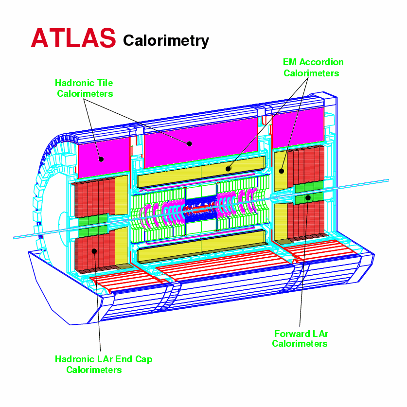
Figure 2.7: Calorimetry in ATLAS: the Electromagnetic Calorimeter is composed of a barrel module (|h|< 1.475) and two end-cap modules (1.375 <|h|< 3.2). The hadronic calorimeter includes the Tile Calorimeter (|h|< 1.7), two Liquid Argon End-cap Calorimeters (1.5 <|h|< 3.2) and two high-rapidity Forward Calorimeters (3.2 <|h|< 4.9).

The ATLAS detector employs a Liquid Argon Electromagnetic Barrel (see Section 2.3.1) module located in the central region of the detector (|h|< 1.475); this module shares the same cryostat with the superconducting solenoid magnet, to reduce the impact of the cooling services on the detector performance. The Hadronic Tile Calorimeter (see Section 2.3.2) is a scintillation calorimeter located around the Electromagnetic Barrel module (|h|< 1.7), to complete the central part of the ATLAS detector.

At higher rapidities, ATLAS employs two identical end-cap sections, each composed of an Electromagnetic End-Cap, a Hadronic End-Cap (see Section 2.3.3) and a Forward Calorimeter. All three subsystems are enclosed in the same cryostat and use the Liquid Argon technology, though they have different absorber structures; in particular the Forward Calorimeter has a higher absorber density and a smaller active volume to withstand high radiation fluxes.

The layout of the Calorimetry system of the ATLAS detector is shown in Figure 2.7.

2.3.1 The Electromagnetic Calorimeter

The Electromagnetic Calorimeter is composed of three parts: an Electromagnetic Barrel (EMB) covering the range |h|< 1.475 and two Electromagnetic End-Cap (EMEC) sections covering the range 1.375 <|h|< 3.2 (see Figure 2.8). Both the EMB and EMEC sections are built according to the same principle: the main building block is a sandwich module of absorber plates and readout electrodes. The absorbers are made of 2.5 mm thick lead plates covered by stainless-steel, and they are folded in the f coordinate (the so-called "accordion" shape, see Fig 2.9); the gap between two adjacent absorbers is 4 mm wide. The readout electrodes are made with copper and Kapton and have the same accordion shape in order to fit in the gaps between the absorber plates; the readout is segmented in the h coordinate by etching the copper electrodes. The accordion shape has two advantages: the electrodes and the absorber plates can be stacked closely together leaving no crack in the detector acceptance along f, and the readout electrodes can be easily accessed from outside the calorimeter, by printing the readout circuitry on the Kapton film, eliminating the need for cabling inside the fiduciary volume. The absorbers and the electrodes are spaced by a plastic honeycombed mesh, and the resulting gaps are filled with Liquid Argon.

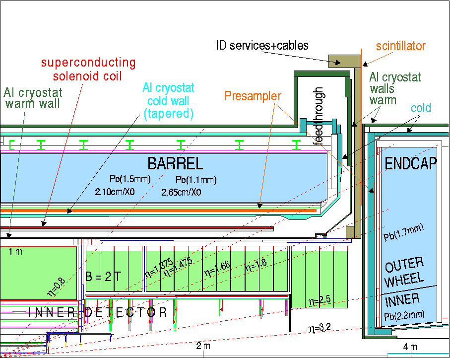
Figure 2.8: Lateral view of the Inner Detector and the Electromagnetic Calorimeter of the ATLAS detector [20].

Both the EMB and the EMEC present three regions with different granularities:

the Sampling 1 (S1 or Strips region) has a very fine granularity (h×f=0.003×0.1) and a depth of 4.3 radiation lengths; this region is used for γ/p⁰ separation;
the Sampling 2 (S2 or Middle region) has a granularity of 0.0250.0245 and a depth of 16X₀; this region is used for precise energy measurement, since most of the energy is deposited here;
the Sampling 3 (S3 or Back region) has a coarse granularity 0.050.0245 and a depth of 2X₀; this region is used to measure the tail of high energy showers which extend past S2; this region is also used to separate between hadronic and electromagnetic showers, since the former deposit a larger amount of energy in S3.

The difference in granularity between the samplings is shown in Figure 2.9. In addition to the three sampling regions, electrode strips are located in front of the accordions at |h|<1.8. These strips form the Pre-sampler region, which is used to correct for the energy deposited in the inner cryostat wall and the Inner Detector.

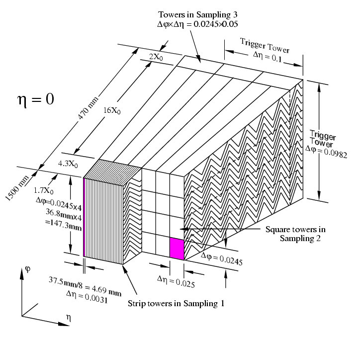
Figure 2.9: Granularity of the LAr calorimeter. Sample 1 is organised in narrow strip cells of 147.34.7 mm to analyse shower shapes in the early development stages and discriminate between γ and p⁰ showers. Sample 2 cells are 0.0250.245 Dh×Df in size and 16 X₀ long and contain most of the deposited energy of the shower. Sample 3 cells are twice the size of a Sample 2 cell (0.050.0245) and are used to identify the broad tails of hadronic showers. The readout lines for all three samples are printed on the Kapton layers of the readout electrodes and carry the signal along the length of the modules to the electronic readout, located behind Sample 3.

Figure 2.10: Optimal filtering of the ionisation signal of the LAr calorimeter: the first five sampling points (shown in the picture) of the signal pulse are inserted in a quadratic function to estimate the total energy [45].

The signal of the Electromagnetic Calorimeter is composed by the electric charge created in the LAr by the incoming particles. The charge is collected by the electrodes and digitized by an ADC. On receiving a signal from the Level 1 Trigger, the ADC samples the ionisation signal in bins of 25 ns; since the typical ionisation peak spans about a hundred of nanoseconds, the signal from several minimum bias events coming from different bunch crosses can pile up in the calorimeter. In order to minimise the noise and signal pile-up, the output signal of the electrodes is shaped by a bipolar circuit; the bipolar shaping function has an area equal to zero, hence the pile-up signal, folded with the shaping function, is zero on average. The residual contributions (the pedestal), can be evaluated and corrected for by reading out the calorimeter with a random trigger.

The signal from the cells of the Electromagnetic Calorimeter is processed by a two-fold calibration: first, the Optimal Filtering algorithm evaluates the height of the ionisation peak from the digitized cell signal; then, the ionisation energy is corrected by a factor that accounts for the effects of the accordion structure of the calorimeter.Both calibration procedures are performed by the trigger softare and are explained in Section 3.4.1.

Test beam results

The validity of the calibration procedure has been proven at the H8 combined test-beam in 2004. A total of seven modules (4 EMB + 3 EMEC) has been tested both in stand-alone mode and combining energy measurement with the hadronic calorimeters. The electron beam ranged from 1 GeV (for material studies, not covered in this chapter) up to 250 GeV. The preliminary results of the test-beam are:

the LAr calorimeter has a linear behaviour over the range 0<E<180 GeV. The deviation from linearity is below 0.1% for E>40 GeV (see Figure 2.11);
the uniformity of the LAr measurements (term c/E for the total energy resolution) for the few modules studied is below the specification limit of 0.7% (See Table 2.1);
the energy resolution for the EMB modules is s(E)/E=8.95%/E+0.33% and s(E)/E=10.35%/E+0.27% for the EMEC modules (see Figure 2.12). These values are within the ATLAS specifications of s(E)/E=10%/E+0.4% for the EMB and s(E)/E=12.5%/E+0.5% for the EMEC.

Module <E> RMS

EMB: (nominal E=250 GeV)

PT13 233.3 0.57%

PT15 236.6 0.64%

EMEC: (nominal E=120 GeV??)

ECC0 119.7 0.58%

ECC1 120.0 0.53%

ECC5 120.2 0.55%

Table 2.1: Uniformity results from the LAr modules at Test-beam 2004. The RMS values measure the spread in response between individual cells of the same module, which amount to the energy resolution term c/E. The difference in the average energy measurement between the EMB modules PT13 and PT15 is due to a difference in temperature of the Liquid Argon between the two test periods. Studies on the effect of temperature on the LAr calorimeter show a variation of about -2%/K in signal, because of density and drift velocity effects [44]. Test beam data taken from [45].

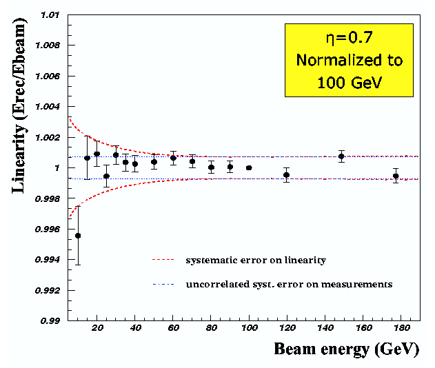
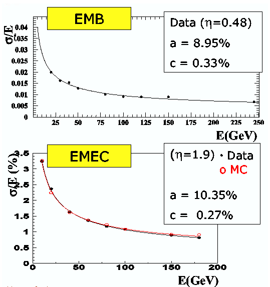
Figure 2.11: Linearity of the LAr calorimeter at the H8 test-beam. Figure taken from [46].

Figure 2.12: Energy resolution of the LAr calorimeter at the H8 test-beam. Figure taken from [46].

In conclusion, the energy measurement performance of the LAr calorimeter has been proven to be inside the TDR specification. Moreover, the LAr calorimeter has been tested in combination with the hadronic tile calorimeter to give an estimate of the overall performance of the ATLAS calorimetry system. The results of the combined performance tests are summarised in Section 2.3.2.

The Electromagnetic End-Cap Calorimeter was tested in combination with the Hadronic End-Cap Calorimeter in the H6 test area. The result of the combined test is outlined in Section 2.3.3.

2.3.2 The Tile Calorimeter

The Hadronic Tile Calorimeter is composed of three cylindrical parts: one barrel sub-detector, covering the rapidity range |h|< 1.0 and two extended barrel wheels, covering the rapidity range 0.8<|h|<1.7 on either side of the barrel. All the sub-detectors are located around the beam axis; the barrel and the two extended barrels are separated by a gap of 600 mm to make space for Liquid Argon distribution pipes (see Figure 2.7).

Each of the sub-detectors is composed by 64 azimuthal wedge-shaped modules (see Figure 2.13): a module is a sandwich-like structure of identical periods stacked next to each other. The period is the basic building block of the calorimeter and consists of four steel plates with gaps to allow the insertion of 3 mm thick plastic scintillator tiles.The tiles are aligned parallel to the LHC beam axis to form 11 tilerows.All the periods which form a module are soldered together by two end-plates at each base of the trapezoid. A barrel module contains 311 periods while an extended barrel module contains 145 periods.

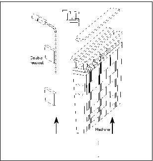
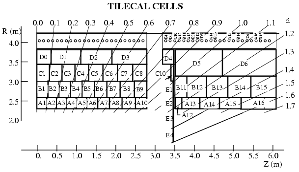
Figure 2.13: Module of the Tile Calorimeter. On the left, the connection between a tile and a PMT via optical fibres is shown. In the Tile Calorimeter each tile is coupled to two PMTs for redundancy. The scintillating tiles slide into the gaps created in the steel matrix of the module (right).

Figure 2.14: Cell grouping in the barrel and end-cap sections of the Tile Calorimeter. The tiles inside the marked areas are assigned to the same cell.

Each scintillator tile is coupled to optical fibres at both free sides; the fibres of several tiles are grouped together to form logical cells. The cell is the readout unit of the Tile Calorimeter: each cell is connected to two photomultiplier tubes (PMT, one for each side of the module) to obtain redundancy; when both photomultipliers are working, the cell signal is the average signal of both photomultipliers; if one photomultiplier is broken, the cell signal is given by the surviving photomultiplier.

The current signal coming from a photomultiplier is sent to a 3in1 board: this board contains a pulse shaper which amplifies the signal and an ADC which converts the pulse in a digital format and sends it to the ROD. The 3in1 board also contains a current integrator which measures the pedestal of the cell and a charge injector to calibrate the ADC.

The cells realise the segmentation of the calorimeter in the R,f,h space: the cells are divided radially in four samples A, B, C, D (see Figure 2.14): Sample A includes tilerows 1-3, Sample B tilerows 4-6 (plus tilerow 7 for the extended barrel), Sample C tilerows 7-9 and Sample D tilerows 10-11 (plus 8-9 for the extended barrel). The cell granularity in the fh plane is 0.1×0.1 for Samples A,B,C while it is 0.1×0.2 for Sample D, which is designed to detect broad shower tails.

All the cells must be calibrated in order to have a uniform response all over the calorimeter; the cell response can be factorised into three contributions: the first contribution is the light response, which describes the light output by the scintillator tiles when a particle shower develops in the calorimeter, convoluted with the efficiency of the readout fibres. The second contribution is the light to charge conversion, which takes place in the photomultiplier tubes, and it is affected by the quantum efficiency and the gain of the photomultipliers. The third contribution is the digitization of the collected charge in the ADC of the readout electronics. The instrumentation of the Tile Calorimeter includes several tools for the calibration and the monitoring of the aforementioned contributions:

a laser system injects light pulses of known intensity in the PMTs, to measure the quantum efficiency and variations in gain due to voltage fluctuations;
a charge injection system located on the 3in1 module injects a fixed charge in the ADC to verify the proper functioning of the digitization process;
all the calorimeter modules are pierced horizontally by pipes who carry a radioactive Cs¹³⁷ source, which emits photons with an energy of 0.662 MeV. As the source travels through the detector, the signal is read out for each individual cell. The gain of the photomultipliers reading the cells is adjusted as to keep signal uniformity within 2%.

Once the calorimeters are calibrated with the on-board systems, the calibration in a test-beam environment can be performed. The aim of this latter calibration is to compare the measurements obtained with the radioactive source with the measurements obtained with the particle beam, in order to extract a conversion factor that correlates the light emitted in the scintillators with the energy of the impinging particle.

The test-beam setup was composed of 4 Tilecal modules --- the pre-production Module 0, one barrel and two end-cap modules --- mounted on a movable support, by means of which the modules could be rotated independently in the h and f coordinates with respect to the test beam. The test beam area was further equipped with:

a Cerenkov counter, needed to identify the particles in the test beam;
three scintillators, used to trigger the system;
two multi-wire Beam Chambers; this chambers measure the path of each particle in the beam. Particles which are inclined with respect to the beam axis are vetoed, since they travel a longer path inside the calorimeter, resulting in an higher than average energy deposition.

Muon beam runs

Muons lose energy almost uniformly inside the Tilecal modules: the average energy deposition of a 180 GeV muon crossing the Tilecal amounts to 1.5 GeV/m. If the modules are rotated to an angle of ±90 with respect to the beam axis, the muon beam crosses perpendicularly all the tiles in the same tilerow; since in this configuration the Cs¹³⁷ pipes are parallel to the beam axis, the response of each tilerow to muons can be compared with the calibration Cesium runs.

Each tilerow is divided into tilerow segments, that are groups of tiles from the same tilerow and the same cell. For each tilerow segment, the energy spectrum of the crossing muons is measured. The spectrum is the combined result of a series of different physical phenomena: first of all the muons deposit inside the tiles an amount of energy that can be modelled by a Landau curve; this energy is converted by the the tiles into visible light that in turn is converted into electrons by the photomultiplier tubes. Both conversion mechanisms are of statistical nature, and their net effect is a Gaussian smearing of the original Landau curve. Thus the muon spectrum in a tilerow segment can be fitted by a Landau distribution convoluted with a Gaussian. For each spectrum curve the truncated mean [47] is extracted by computing the mean value of the distribution for energy values up to 5.5 times the energy of the Most Probable Value (MPV). The truncated mean is a valid statistic estimator of the energy distribution and reduces the effects of fluctuations in the Landau tail; moreover, since the truncated mean is an additive variable, the truncated means of different tilerow segments can be added together to form the estimated mean energy deposition of a calorimeter cell.

The uniformity of response of tilerow segments was evaluated by computing the RMS of the set of segments' responses for each module. All the tested modules presented an RMS below 5% of the average response, and the mean RMS for all modules was about 3.8% [47]; the Cesium calibration run, in comparison, resulted in a mean RMS of 2.7%.

The calibration constants obtained in the muon calibration runs are transfered to all the modules in the following way: the calibration constants from a reference module r are used as a fixed parameter. Then, for each other module i, and for each tilerow segment j, the expected muon response F is correlated to the measured muon response in the reference module by[47]:

F_expected^muon(i,j)=

F^Cesium(i,j)

F^Cesium(r,j)

× F_measured^muon(r,j).

This way, the calibration constants are obtained for modules that are not tested with a muon beam.

Combined barrel test results

The energy measurements of pion beams in the Electromagnetic Calorimeter and the Hadronic Tile Calorimeter were combined at the H8 test beam to evaluate the energy resolution of the barrel calorimetry section of the ATLAS detector. The energies measured in the two subsystems are added using the following empirical formula [49]:

E=a₁E_Tile+E_LAr+a₂×a₁E_Tile1E_LAr3+a₃E_LAr²

where a₁ represents the inter-calibration factor between the LAr and the Tile calorimeters (set equal to 1 for this study); the term with the square root corrects for the energy loss occurring in the LAr cryostat, and it is dependent on the energy measured in the calorimeter samples immediately before and after the cryostat --- that is, the last LAr sample E_LAr3 and the first Tilecal sample E_Tile1. The last term a₃E_LAr² is a correction for the non-compensating nature of the LAr calorimeter.

The resolution for this combined reconstruction is summarised on Table 2.2. These results are worse than benchmark results obtained in 1996 --- s(E)/E=59.5%/E+1.8%⊕2.1%/E for |h|~0.2 --- and the causes have not been yet identified at the time of writing [49]. However, the energy resolution might receive a beneficial contribution from the use of the cluster weighting technique, which has been tested in the end-cap section with encouraging results (see Section 2.3.3).

h a (%) b (%) c (%)

0.2 65±4 4.3±0.2 2.7±0.2

0.25 66±4 2.7±0.2 3.3±0.2

0.35 68±4 3.1±0.2 3.2±0.2

0.45 54±4 3.9±0.1 2.9±0.1

0.55 50±4 4.3±0.2 3.3±0.1

Table 2.2: Parameters of the energy resolution s/E=a/E⊕b/E⊕ c for combined Liquid Argon/Tilecal measurements of pions at the H8 test-beam. Table taken from [49].

2.3.3 The Hadronic End-Cap Calorimeter

The Hadronic End-Cap Calorimeter (HEC) is a Liquid Argon calorimeter, made of two end-cap sections. Each of the two end-caps is composed by two independent wheels, made of a stack of flat copper plates. The first wheel stacks 25 copper plates of 25 mm thickness (with the exception of the first plate, which is 12.5 mm thick); between two consecutive plates there is a gap of 8.5 mm, where three electrodes are placed. The second wheel is built in the same way, with 17 copper plates of 50 mm.

The electrodes are made of a highly resistive plastic plate, sandwiched between two conductive Kapton layers; the middle electrode has an extra inner layer, made of copper tiles (see Figure 2.15). All three electrodes are connected to high voltage, and the copper tiles of the middle electrode are connected to a readout circuit. The middle electrode and the two outer electrodes form an Electrostatic Transformer: the 8.5 mm LAr gap between the absorber plates is separated in four, isolated 1.8 mm gaps; smaller gaps require a lower operating voltage and minimise the risk of high ion build-up and discharge currents.

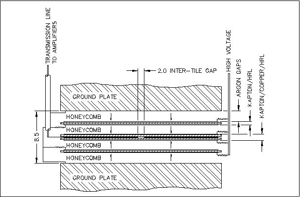
Figure 2.15: The Electrostatic Transformer of the Hadronic End-Cap Calorimeter. Three electrodes divide the 8.5 mm gap into four 1.8 mm gaps. The four gaps are electrically isolated by the highly resistive layer of the electrodes. The Kapton layers of the electrodes act as capacitors to couple electrostatically the gap and carry high voltage to generate the electric field in which the ionisation charges drift. The inner copper layer of the middle electrode is used to read out the collected charge [50].

The readout copper tiles of the middle electrodes are segmented with a granularity of Dh×Df=0.1×0.1; the charge collected from each segment is sent to a pre-amplifier/summer circuit. A calorimeter cell is formed by summing signals from projective segment towers spanning several LAr gaps. The depth of a cell depends from its position in the HEC: the first wheel is divided in a sampling region with 8-gaps-deep cells (HEC1 Front) and a sampling region with 16-gaps-deep cells (HEC1 Back); the second wheel is divided in two equal sampling regions with 8-gaps-deep cells (HEC2 Front and HEC2 Back). The signal from a HEC cell is calibrated by the trigger system (see Section 3.4.1).

Combined end-cap test results

The main obstacle to an accurate measurement of the energy of hadronic showers is the presence of invisible energy; in a Liquid Argon calorimeter, the energy of the incoming particles is proportional to the charge created in the Argon volume: charged particles ionise the Argon atoms or emit bremsstrahlung photons, which can excite the atoms or produce an electron/positron pair; light neutral particles (such as pions) can decay in a photon pair, giving rise to an electromagnetic shower. Hadronic particles lose most of their energy in a hard interactions with the absorber, either exciting or breaking its nuclei; in either case, only a fraction of the lost energy creates a ionisation charge, while the rest is not visible by the calorimeter. Luckily, it is possible to compensate the invisible energy of the shower by applying to the measured energy a weight given by:

w=c₁exp

/

|
|

\

-c₂

E

V

\
|
|

/

+c₃,

where E/V is the density of the measured energy. The coefficient c₃ is close to unity, which means that for high energy densities the electromagnetic response is an adequate measure of the shower energy, and invisible energy is negligible.

The ATLAS approach to hadronic energy calibration is based on the weighing technique developed at the H1 experiment. The ATLAS algorithm uses the weight equation described above; since the weight to be used is different for the electromagnetic and hadronic parts of the shower, it is necessary to introduce an algorithm to split jet clusters into sub-clusters, and to classify sub-clusters as hadronic or electromagnetic according to their energy density [51]. The ATLAS calorimeters are non-compensating, thus high energy densities are associated with electromagnetic sub-clusters, while low energy densities with hadronic ones. The splitting algorithm works on topological clusters, which are clusters crossing sub-detector boundaries --- for the end-cap region, topological clusters are built by joining neighbouring and overlapping cells from the Electromagnetic End-Cap, the Hadronic End-Cap and the Forward Calorimeter.

The algorithm builds a list of seed cells which are local maxima. Neighbouring cells are added to to the seed cells to form a sub-cluster if their signal is three times higher than the sigma of the average noise level; sub-clusters are never merged if they belong to different maxima. Once all sub-clusters are identified, for each sub-cluster the energy density is calculated and the weight is applied.

This technique has been tested at the H6 test beam facility. The setup included an Electromagnetic End-Cap module, one HEC1 wheel and half (8 gaps instead of 16) HEC2 module. Different particle beams were used: e±, µ± and p±, with energies ranging from 6 to 200 GeV [51]. The electromagnetic response for both the EMEC and the HEC was measured in the electron runs, and the leakage for electromagnetic showers was estimated by a GEANT4 simulation of the setup.

For pion runs, both the splitting algorithm and the weighing technique were used: for each incoming particle, a topological cluster was built using the EMEC and HEC cells; the cluster was split into electromagnetic and hadronic sub-clusters. For each sub-cluster and for each sub-detector, the weights were found by a c² fit; the constraint on the fit required the sum of the weighted energy of the sub-detectors plus the leakage to be equal to the nominal beam energy:

∑

sub-clusters

∑

detectors

(

E_beam-E_leak-E_{other detector}^{(weighted+leak)}-E_weighted

)

²

s²

.

The weights extracted analysing the test beam data are shown of Figure 2.16; the weight dependence on energy density was compared with GEANT3 and GEANT4 simulation of the test setup: the Montecarlo description simulates the data quite well, though at low energies the shower leakage is underestimated by a few percent [51]. The energy scale correction brings the resolution of the combined EMEC-HEC measurements to

s(E)

E

=

84.1%

E

⊕0.3%

with a constant noise term of 1-1.5 GeV. The weighting technique improves significantly the energy resolution, as shown in Figure 2.17.

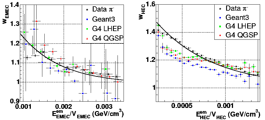
Figure 2.16: Correction weights to the measured visible energy density for the EMEC (left) and HEC (right) modules tested at the H6 test-beam. The data agrees with different Montecarlo simulations. Figure taken from [51].

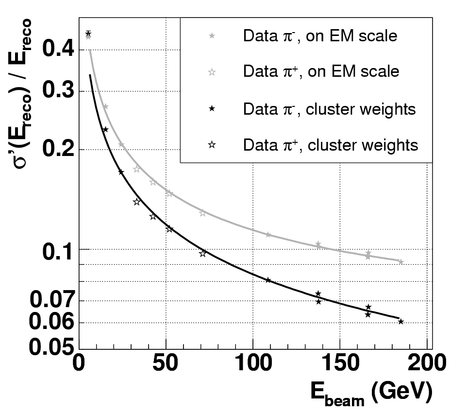
Figure 2.17: Resolution of the combined EMEC/HEC calorimetry system at H6. The weighted data (in black in the figure) exhibits a better resolution than the uncorrected data (in gray). Figure taken form [51].

2.4 The Muon Spectrometer

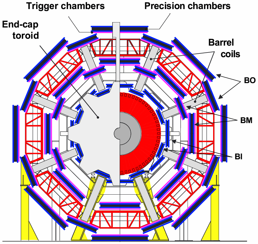
Figure 2.18: Cross-section of the barrel of the ATLAS Muon Spectrometer. The MDT precision chamber are organised in projective towers of three layers ("stations") each. The three stations are denominated "barrel inner" (BI) "barrel middle" (BM) and "barrel outer" (BO). A third letter is added to the denomination to identify large (L) or small (S) chambers --- BOL chambers were built at NIKHEF. The trigger chambers share the mechanical support with the MDT chambers: two trigger RPC chambers are mounted per BM MDT chamber, and one RPC chamber is mounted per BO MDT chamber. The Muon Spectrometer is immersed in a 4 T toroidal magnetic field, generated by eight air-core coils and two end-cap toroids (partially seen in figure).

The ATLAS Muon Spectrometer is based around a large toroidal "air-core" magnetic field. As seen in Section 1.7.6, the momentum resolution of the spectrometer is inversely proportional to the lever arm BL and it is increased by multiple scattering in passive material. The absence of an iron yoke in the ATLAS spectrometer minimises the amount of multiple scattering, facilitating an excellent resolution.

The magnetic field of the Muon Spectrometer is divided into several regions:

the barrel (|h|£1.0), with a 4.4 T toroidal magnetic field;
two end-caps (1.4£|h|£2.7), with a 4.6 T magnetic field;
two "transition regions" (1.0£|h|£1.4) where the magnetic field is the sum of the barrel and end-cap magnetic fields.

The instrumentation of the Muon Spectrometer is composed of trigger chambers and precision chambers. Trigger chambers are fast detectors who perform coarse measurements of the muon momentum; precision chambers, instead, measure momenta with a better resolution but are much slower, so the data has to be stored in memory buffers and retrieved upon request from the trigger (see Chapters 3 and 4).

ATLAS uses two types of precision chambers in the spectrometer: Monitored Drift Tube (MDT) chambers and Cathodic Strip Chambers (CSC). The trigger system of the spectrometer uses Resistive Plate Chambers (RPC) and Thin Gap Chambers (TGC).

In the barrel region, MDT chambers and RPC chambers are situated in three concentric layers ("stations"), at 5, 7.5 and 10 m of radius from the beam axis. All the chambers are aligned to form projective towers in the hf space; two MDT chambers (and the relative RPC chambers) are taken from each station, for a total of six MDT chambers for each tower.

In the end-caps and the transition regions, the Muon Spectrometer is instrumented with MDT and TGC chambers, arranged in three wheels; at high pseudorapidities ( 2£|h|£2.7), where high counting rates are expected, CSC chambers are mounted between the calorimeter end-caps (see Section 2.3.3) and the end-cap magnets.

CSC MDT RPC TGC

Number of chambers 32 1194 596 192

Number of channels 67000 370000 355000 440000

Area coverage (m²) 27 5500 3650 2900

Table 2.3: Instrumentation of the Muon Spectrometer [52].

TGC chambers

Thin Gap Chambers are gaseous detectors composed by an array of Tungsten anodes wire and segmented graphite cathodes. The spacing between the wires and the cathodes is smaller (1.4 mm) than the intra-wire spacing (1.8 mm), hence the denomination Thin Gap.

The signal in the TGC is generated by ionisation charge created in the gas; the electrons are accelerated by the electric field of the wires and produce secondary charges (the so-called avalanche charge) which is collected on the wires, giving rise to a fast current pulse signal; the avalanche induces an oppositely charged pulse on the cathodes. Since the cathodes are segmented orthogonally to the anode wires, TGC chambers can measure particle tracks in two coordinates. TGC chambers are built in doublets and triplets, that is chambers with respectively two and three layers of cathodes/wires, separated by cardboard honeycomb.

TGC chambers are filled with a gas mixture composed of 55% CO₂ and 45% n-pentane. The chambers are working in the gas saturation regime, which gives a signal which is very stable in amplitude and independent from the incidence angle of the crossing particles. The small size of the drift cell and the gas choice guarantee a short drift time (typically less than 25 ns), which is important in order to discriminate particle tracks from different bunch crosses. The readout electronics of the TGC chambers matches hits from the TGC layers inside a coincidence window to extract a trigger signal (see Section 3.4.2). The performance of the TGC readout was tested at H8: by adjusting the delay and width of the coincidence window, the TGC trigger can obtain a trigger efficiency of 98%, with 2% of bunch mismatch (see Figure 2.19).

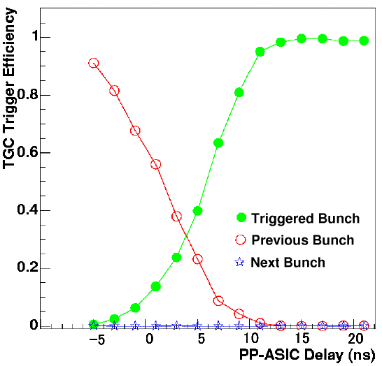
Figure 2.19: Efficiency of the TGC trigger. The TGC readout electronics matches hits inside a programmable coincidence window. The window has two important parameters: width, which is set by default at 25 ns, and the delay, which accounts for the drift time in the drift cell. By adjusting the delay, an efficiency of 98% can be achieved, while limiting pile-up from out-of-time tracks at about 2% [55].

RPC chambers

The Resistive Plate Chamber is a gaseous detector composed of two gas gaps. Each gap is made of two Bakelite slabs separated by polycarbonate spacers. The 2 mm gap between the slabs is filled by a non-flammable gas mixture --- 97% tetrafluoroethane (C₂H₂F₄) - 3% isobutane (C₄H₁₀). The Bakelite slabs are coated with a graphite paint which is connected to the HV supply, generating an uniform electric field of 4.5 kV/mm inside the gap. The slabs are capacitively coupled with two aluminium pickup plates, which are segmented in orthogonal directions. The gas is operating in the saturation regime, and the charge deposited by incoming particles gets multiplied by the avalanche mechanism before being collected on the slabs. The collected charge induces a charge pulse in the pickup plates, which is read out by the chamber's electronics. The pickup plates are segmented in 30-40 mm wide strips, separated by a 2 mm gap and a 0.5 mm grounding strip to prevent cross-talk. For each gas gap, one series of pickup strips is oriented in the azimuthal direction --- measuring the particle track in the bending plane --- and the second series of strips is oriented in the h direction, measuring the track in the second coordinate. The crossing point of the incoming particles is measured by calculating the centroid of the charge deposition on the pickup strips, and the typical spatial resolution is about 1 cm for both coordinates.

The Muon Spectrometer employs three layers of RPC chambers: two layers of RPC chambers are mounted on the middle MDT stations and one layer is mounted on the outer MDT stations (see Figure 2.18).

CSC chambers

The CSC chamber is a proportional multi-wire chamber with segmented readout cathodes. The drift cell of the CSC chamber is symmetric, as the distance between the anode wires and the cathodes is equal to the intra-wire distance (2.54 mm). The cathodes are segmented in 1 mm strips, orthogonal to the anode wires, allowing to measure the crossing point of incoming muon with a resolution of 60 µm--- the CSC chambers are used in the "point and angle" technique (see Section 1.7.6), thus they do not perform track measurements, but point measurements. The CSC chambers are positioned in the end-cap section of the spectrometer, where the high flux of particles needs detectors with a low occupancy; the maximum drift time of CSC chambers is 30 ns, reducing the risk of pile-up between consecutive bunch crossings.

MDT chambers

MDT chambers are drift chambers composed by two multi-layers of drift tubes --- each multi-layer is composed by three or four layers of tubes. The two multi-layers are connected by a support structure (the spacer) made of two long beams and three cross plates (see Figure 2.20). The difference between MDT chambers and traditional drift chambers is that each drift cell is enclosed in an aluminium tube, which provides grounding to the drift cell as well. The tubes provide mechanical stability to the chambers, which can be up to 5 m long; moreover, the end-plugs of the tubes provide a high-precision reference surface which guarantees the positioning of the sense wires within 20 µm of the design location.

The drift tubes are made aluminium cylinders with a 400 µm thick wall and 30 mm of inner bore. Each tube contains a 50 µm Copper-plated Tungsten-Rhenium wire which is kept in position by a precision wire locator inserted in the tube end-plugs [56]. The tubes are filled with a gas mixture --- 97% Ar, 3% CO₂, at 3 bars --- which guarantees an almost linear relation between track position and drift time. Particle tracks in the MDT chambers are measured by time-stamping the arrival of ionisation charges on the anode wire, and converting the timestamp into a radius using the drift time relation. The electronic systems responsible for the timestamping and the retrieval of MDT data are described in Chapter 4.

In order to obtain the maximum resolution from the MDT tubes, the anode wire should ideally be placed along the tube axis; however, because of the effect of gravity, the centre of the wire sags and it is displaced by several hundreds of microns from the nominal position. To compensate this effect, the weight of the cross-plates of the MDT chambers exercise a pull on the long beams of the support structure, which deforms the tubes in a way which is similar to the gravitational sag of the wire. The net effect of the deformation is to compensate the wire sag, keeping the maximum displacement of the wire from the nominal position below 100 µm [52]. The deformation of the the MDT chambers is constantly kept under observation by the infrared optical system RASNIK, developed at NIKHEF. The monitoring of the drift tubes permits to apply offline correction to the track measurements, whenever the tubes might be deformed by gravitational pull, thermal excursions or magnetic force, or when the positioning of the MDT chambers in the Spectrometer is different from the nominal values. The design resolution for a single MDT tube is 80 µm; to measure a track position, the MDT chambers combine data from 6 to 8 tubes, resulting in a final track resolution of about 30 µm.

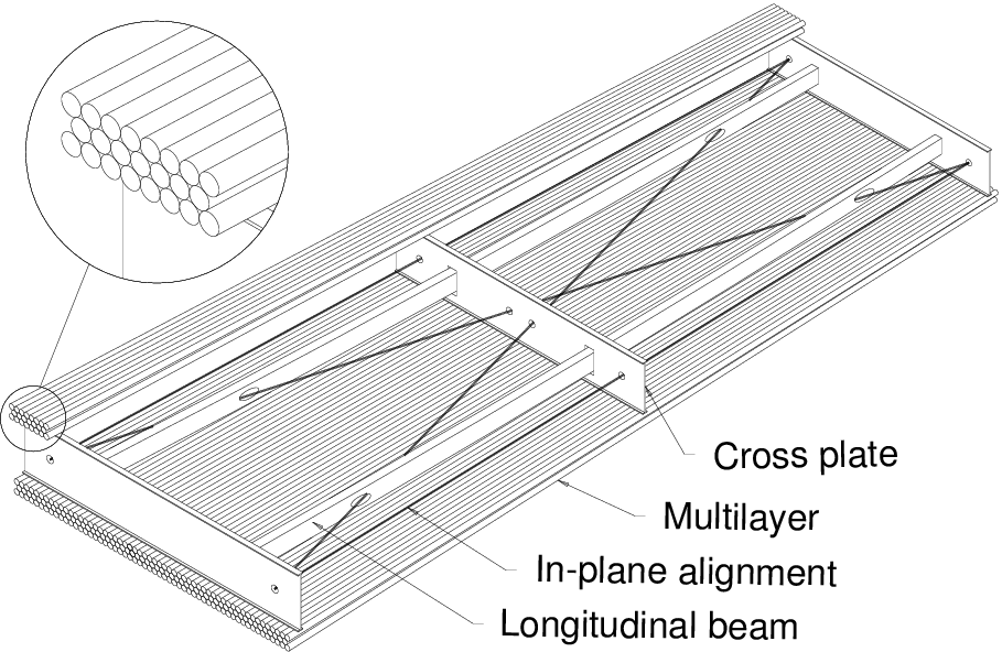
Figure 2.20: Structure of a MDT chamber. Each multi-layer is composed by three or four layers of drift tubes glued together. The two multi-layers are connected to a support structure made of two long beams and three cross-plates. The weight of the cross-plates deforms the tubes, counterbalancing the gravitational sag of the anode wires. The deformation is monitored by the optical RASNIK in-plane alignment system.

2.4.1 Combined test results

During the H8 test beam the MDT chambers were subjected to several tests, including:

thermal deformations of the chambers and offline corrections;
efficiency of the alignment system and corrections of MDT misplacements;
effects of gas pressure and composition on the resolution;
aging of MDT chambers.

The integration of the Muon Spectrometer with other ATLAS detectors in the Combined Test Beam allowed for an extension of the test program; since the muons leave a measurable signal across all the detectors, they make cross-checks between all detectors possible.

One of such tests, still in the preliminary phases [57], aims to evaluate the energy loss of muons in the ATLAS calorimeter by measuring the difference in the momentum of muons in the Inner Detector and in the Muon Spectrometer. The test was performed using muons with energies between 180 and 350 GeV; in the Inner Detector mock-up, the muon momenta can be measured by measuring the deflection of muons in the ID magnet; given the equation $\Delta \theta \simeq {\frac {0.3BL}{p}}$ and with a magnetic field of 0.4 Tm, a 250 GeV muon is deflected by about 0.480 mrad by the magnet. By design, the TRT should be able to measure track angles down to a resolution of 0.160 mrad; however, at the time of writing, problems in the calibration of the TRT resulted in a resolution of the same order of the deflection, degrading the measurement. The muon momentum was evaluated by measuring the angle between the TRT tracks and the tracks measured by the Beam Chambers. The muon momentum spectrum measured in the TRT is shown in Figure 2.21; the measured momentum underestimates the actual muon momentum.

In the Muon Spectrometer, the muon momenta are evaluated in a similar way, by measuring the difference in track angles before and after the magnet. Using the same equation used for the Inner Detector, with a magnetic field of 2 Tm, one obtains a deflection of about 2.4 mrad for 250 GeV, which is the central value for the beam energy range of 180-350 GeV. The difference in angle measured at the test-beam was 2.37±0.87, compatible with the expected result; the spectrum of the measured angles can be converted to a momentum spectrum (see Figure 2.22) which is consistent with the nominal energy of the muon beam.

The difference in the momentum of individual muons measured in the TRT and MDT can be plotted against the energy lost by the muons in the LAr calorimeter. Supposing the detectors are perfectly calibrated, the difference between the momenta measured in the TRT and the MDT should be equal to the energy loss. However, since at the time of writing the TRT was not properly calibrated, the difference in momentum exhibited a large offset of about 150 GeV; despite this offset, the measured momentum difference has a linear dependence with respect to the calorimeter energy. The test beam data can be fitted with a straight line, with a slope of 1.107±0.412 (see Figure 2.23) indicating that, despite the poor calibration and the large offset, it is still possible to correct for energy losses in the calorimeter.

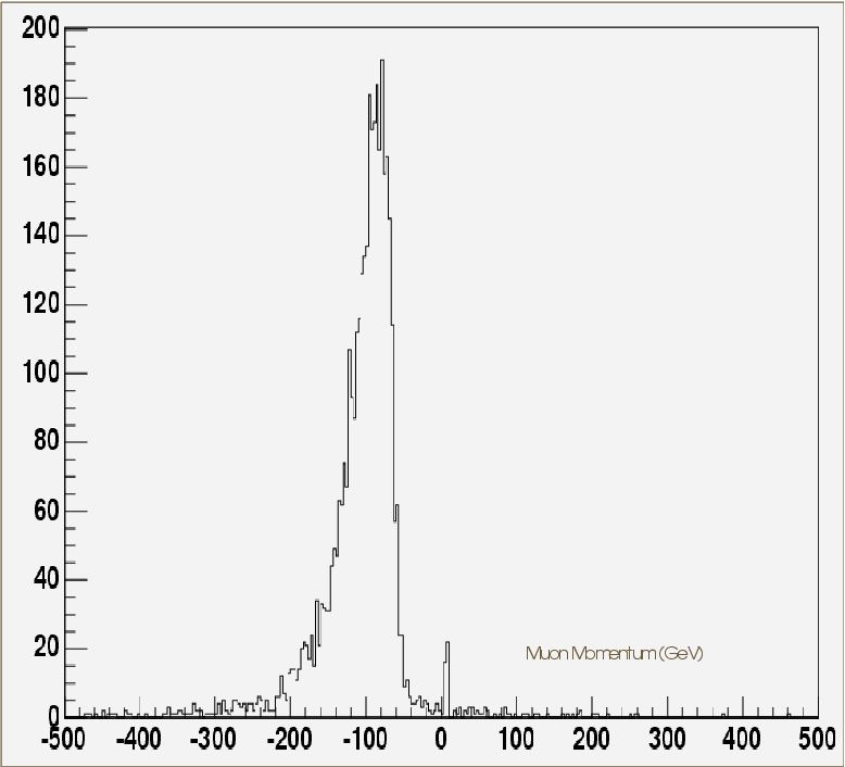
Figure 2.21: Momentum spectrum of the muon beam at H8, measured by comparing the difference of angle of muon tracks in Beam Chambers and the TRT modules. The resulting spectrum underestimates the momentum of the muon beam, because of inaccuracies in the TRT calibration. Figure taken from [58].

Figure 2.22: Momentum spectrum of the muon beam at H8, evaluated by measuring the angle of deflection of muon tracks in MDT chambers under the effect of a magnetic field. The nominal beam energy was 180-350 GeV. Figure taken from [58].

Figure 2.23: Effect of energy loss in the calorimeter on muon tracks. The difference in momenta between the TRT and the MDT is plotted against the energy loss in the calorimeter. Figure taken from [58].

1: The staging of elements of the Inner Detector reduces the coverage to about |h|<1.7 in the initial ATLAS layout
2: Kapton is a flexible polymide film, produced by DuPont, which has several industrial uses. In ATLAS, Kapton is used as a pliable support for electronic circuits and cabling.

--Barison 14:50, 19 Jul 2005 (MET DST)

Chapter II

Contents