Difference between revisions of "Dark count dependence on temperature"
(→Analysis: Add Poisson) |
(→Analysis: Add rest of analysis) |
||
| Line 14: | Line 14: | ||
== Analysis == | == Analysis == | ||
| − | For each temperature, we count the peaks in each recorded waveform. Because there is a lot of high-frequency noise on top of the signal, we low-pass filter the signals before peakfinding. The result is shown in Figure 3 for the signal in Figure 2. Even though there is noise, the filtering and peak finding steps manage to identify the correct signal peaks. In Figure 3, we | + | For each temperature, we count the peaks in each recorded waveform. Because there is a lot of high-frequency noise on top of the signal, we low-pass filter the signals before peakfinding. The low-pass filter is a Butterworth filter with a cut-off frequency of 10MHz and order 1. The peakfinding uses a minimal height of 0.02, a width of 180, and a prominence of 0.05. The result is shown in Figure 3 for the signal in Figure 2. Even though there is noise, the filtering and peak finding steps manage to identify the correct signal peaks. In Figure 3, we see that this waveform counts 6 peaks. Figure 4 shows a histogram of counts for all 1500 waveforms for 1 degree Celcius. The distribution resembles a Poisson distribution fairly well. Therefore, we can use Poisson statistics to calculate the uncertainty. In Figure 5 you can see the resulting plot. Here we show the average number of peaks per waveform per temperature. The counts increase with temperature. We can convert these counts to a rate per second and fit the theoretical curve to the data. The final result is shown in Figure 6. We fitted Formula 1 to the measured points. From the best fit parameters we can obtain information about the band gap energy Eg. |
| + | [[File:Afbeelding.png|left|thumb|Formula 1: Dark count probability]] | ||
== Conclusions == | == Conclusions == | ||
| Line 20: | Line 21: | ||
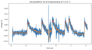
[[File:Filteredandpeaks.png|left|thumb|Figure 3: In blue the raw data, which is also in Figure 2. In orange the low-pass filtered data, and in red the peaks.]] | [[File:Filteredandpeaks.png|left|thumb|Figure 3: In blue the raw data, which is also in Figure 2. In orange the low-pass filtered data, and in red the peaks.]] | ||
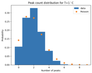
[[File:1degrees Poisson.png|left|thumb|Figure 4: Histogram of the counts for all 1500 waveforms for 1 degree Celcius. In orange a Poisson distribution is shown with the same average as the blue histogram. The two distributions are similar.]] | [[File:1degrees Poisson.png|left|thumb|Figure 4: Histogram of the counts for all 1500 waveforms for 1 degree Celcius. In orange a Poisson distribution is shown with the same average as the blue histogram. The two distributions are similar.]] | ||
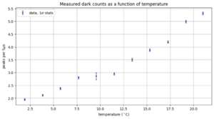
| + | [[File:Darkcounts.png|left|thumb|Figure 5: The darkcounts per 5 μs with 1σ Poisson errors.]] | ||
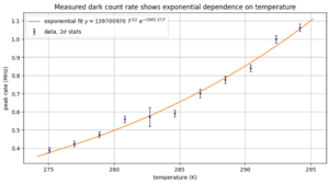
| + | [[File:Fit.png|left|thumb|Figure 6: Dark count rate in MHz and temperature in Kelvin, with in orange a fit to the data.]] | ||
Revision as of 16:31, 8 February 2023
The dark count rate depends on temperature. We use a peltier element and a dark box to quantify this relationship.
Setup
@Vikas: can you update this?
Measurements
We took dark count measurements at 12 different temperatures.
T = [9.565, 7.664, 1.915, 3.823, 11.484, 5.735, 17.256, 15.32, 13.405, 19.185, 21] degrees Celcius.
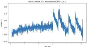
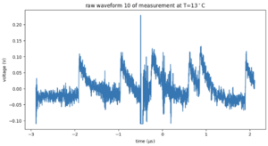
For each temperature, around 1500 waveforms were recorded with an oscilloscope. Each waveform is 5 microseconds. You can clearly see the single p.e. peaks already in the raw waveform shown in Figure 1. In Figure 2, a waveform with electronic noise is shown. For 9 degrees Celcius, we have only a few waveforms available.
Analysis
For each temperature, we count the peaks in each recorded waveform. Because there is a lot of high-frequency noise on top of the signal, we low-pass filter the signals before peakfinding. The low-pass filter is a Butterworth filter with a cut-off frequency of 10MHz and order 1. The peakfinding uses a minimal height of 0.02, a width of 180, and a prominence of 0.05. The result is shown in Figure 3 for the signal in Figure 2. Even though there is noise, the filtering and peak finding steps manage to identify the correct signal peaks. In Figure 3, we see that this waveform counts 6 peaks. Figure 4 shows a histogram of counts for all 1500 waveforms for 1 degree Celcius. The distribution resembles a Poisson distribution fairly well. Therefore, we can use Poisson statistics to calculate the uncertainty. In Figure 5 you can see the resulting plot. Here we show the average number of peaks per waveform per temperature. The counts increase with temperature. We can convert these counts to a rate per second and fit the theoretical curve to the data. The final result is shown in Figure 6. We fitted Formula 1 to the measured points. From the best fit parameters we can obtain information about the band gap energy Eg.
