Difference between revisions of "Dark count dependence on temperature"
(→Analysis: Add Poisson) |
|||
| Line 14: | Line 14: | ||
== Analysis == | == Analysis == | ||
| − | For each temperature, we count the peaks in each recorded waveform. Because there is a lot of high-frequency noise on top of the signal, we low-pass filter the signals before peakfinding. The result is shown in Figure 3 for the signal in Figure 2. Even though there is noise, the filtering and peak finding steps manage to identify the correct signal peaks. | + | For each temperature, we count the peaks in each recorded waveform. Because there is a lot of high-frequency noise on top of the signal, we low-pass filter the signals before peakfinding. The result is shown in Figure 3 for the signal in Figure 2. Even though there is noise, the filtering and peak finding steps manage to identify the correct signal peaks. In Figure 3, we count 7 peaks. Figure 4 shows a histogram of counts for all 1500 waveforms for 1 degree Celcius. The distribution resembles a Poisson distribution fairly well. Therefore, we can use Poisson statistics to calculate the uncertainty. |
== Conclusions == | == Conclusions == | ||
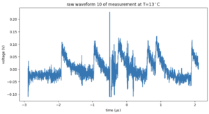
[[File:Noisywaveform.png|left|thumb|Figure 2: Raw waveform at 13 degrees showing noise.]] | [[File:Noisywaveform.png|left|thumb|Figure 2: Raw waveform at 13 degrees showing noise.]] | ||
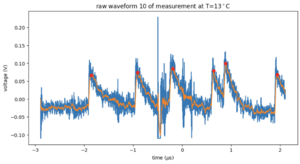
| − | [[File:Filteredandpeaks.png|left|thumb|Figure 3: | + | [[File:Filteredandpeaks.png|left|thumb|Figure 3: In blue the raw data, which is also in Figure 2. In orange the low-pass filtered data, and in red the peaks.]] |
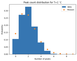
| + | [[File:1degrees Poisson.png|left|thumb|Figure 4: Histogram of the counts for all 1500 waveforms for 1 degree Celcius. In orange a Poisson distribution is shown with the same average as the blue histogram. The two distributions are similar.]] | ||
Revision as of 16:19, 8 February 2023
The dark count rate depends on temperature. We use a peltier element and a dark box to quantify this relationship.
Setup
@Vikas: can you update this?
Measurements
We took dark count measurements at 12 different temperatures.
T = [9.565, 7.664, 1.915, 3.823, 11.484, 5.735, 17.256, 15.32, 13.405, 19.185, 21] degrees Celcius.
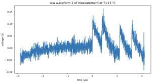
For each temperature, around 1500 waveforms were recorded with an oscilloscope. Each waveform is 5 microseconds. You can clearly see the single p.e. peaks already in the raw waveform shown in Figure 1. In Figure 2, a waveform with electronic noise is shown. For 9 degrees Celcius, we have only a few waveforms available.
Analysis
For each temperature, we count the peaks in each recorded waveform. Because there is a lot of high-frequency noise on top of the signal, we low-pass filter the signals before peakfinding. The result is shown in Figure 3 for the signal in Figure 2. Even though there is noise, the filtering and peak finding steps manage to identify the correct signal peaks. In Figure 3, we count 7 peaks. Figure 4 shows a histogram of counts for all 1500 waveforms for 1 degree Celcius. The distribution resembles a Poisson distribution fairly well. Therefore, we can use Poisson statistics to calculate the uncertainty.


