Difference between revisions of "Chapter V"
| Line 1: | Line 1: | ||
| − | < | + | <!--TOC chapter Event Generation and Reconstruction--> |
| − | The startup of the LHC machine will take place in April 2007, and few months will pass before a data sample is ready for analysis. In the meantime, simulations of | + | <H1>Chapter 5 Event Generation and Reconstruction</H1><!--SEC END --> |
| − | + | ||
| − | <UL><LI>Monte Carlo Event Generators, which compute the matrix elements of the partonic scattering at fixed order; | + | The startup of the LHC machine will take place in April 2007, and few months will pass before a data sample is ready for analysis. In the meantime, simulations of the physics processes can be used to tune the physical analysis and forecast the results. Simulation software is composed by a chain of different elements: |
| + | <UL><LI>Monte Carlo Event Generators, which compute the matrix elements of the partonic scattering at fixed order; | ||
<LI>Parton Shower Algorithms, which hadronise the scattered partons and simulate the emission of soft gluons and photons in the non-perturbative regime; | <LI>Parton Shower Algorithms, which hadronise the scattered partons and simulate the emission of soft gluons and photons in the non-perturbative regime; | ||
| − | <LI>Detector Simulations, which reproduce the effects of the finite resolution of the detector instrumentation on the observables. Detector simulations are of two | + | <LI>Detector Simulations, which reproduce the effects of the finite resolution of the detector instrumentation on the observables. Detector simulations are of two types: |
| − | |||
<UL><LI> | <UL><LI> | ||
Fast Detector Simulations, where the momenta of the particles are convoluted with parametrised smearing functions; | Fast Detector Simulations, where the momenta of the particles are convoluted with parametrised smearing functions; | ||
| − | <LI>Full Detector Simulations, where the interaction of particles with the detector is simulated at the microscopic scale --- resulting in, for example, realistic | + | <LI>Full Detector Simulations, where the interaction of particles with the detector is simulated at the microscopic scale --- resulting in, for example, realistic electromagnetic shower shapes, multiple scattering, etc. |
| − | |||
</UL> | </UL> | ||
</UL> | </UL> | ||
| − | The ATLAS collaboration organizes every two years a conference to discuss issues and results of the prospective physics analyses. In preparation for the 2005 | + | The ATLAS collaboration organizes every two years a conference to discuss issues and results of the prospective physics analyses. In preparation for the 2005 conference, held in Rome, a sample of five million events was produced with full detector simulation. As member of the ATLAS Top Physics Working Group, I had the task to generate a fraction of this sample, dedicated to single top production. In this Chapter I will outline the software framework for the simulation of physics processes in ATLAS, the systematic uncertainties in the use of fixed-order Monte Carlo generators, and the data sample for the ATLAS Physics Workshop 2005.<BR> |
| − | |||
| − | |||
| − | |||
<BR> | <BR> | ||
<!--TOC section Monte Carlo Generators--> | <!--TOC section Monte Carlo Generators--> | ||
| − | <H2> | + | <H2>5.1 Monte Carlo Generators</H2><!--SEC END --> |
<!--TOC subsection TopReX--> | <!--TOC subsection TopReX--> | ||
| − | <H3> | + | <H3>5.1.1 TopReX</H3><!--SEC END --> |
| − | The Monte Carlo generator was written with the specific intent of treating top production and decay []. provides production processes not implemented in popular | + | The Monte Carlo generator was written with the specific intent of treating top production and decay []. provides production processes not implemented in popular Monte Carlo packages such as <FONT COLOR=navy>Pythia</FONT> or <FONT COLOR=navy>Herwig</FONT>. In particular, implements both the Feynman diagrams associated with W-gluon fusion and takes into account the spin polarization of the decay products of the top quark.<BR> |
| − | |||
| − | |||
<BR> | <BR> | ||
| − | As alread explained in Section | + | As alread explained in Section 1.3.2, the W-gluon fusion channel is described by the interference of LO and NLO diagrams. The NLO diagram features an extra <I>b</I> quark in the final state; however, this extra quark could be produced at LO by initial state radiation. In order to avoid the double-counting of events and produce a cross-section consistent with theory, introduces two cut-off parameters <I>k</I><FONT SIZE=2><SUB>0</SUB></FONT><U>~</U>20 GeV and <I>p</I><FONT SIZE=2><SUB>0</SUB></FONT><U>~</U>10 GeV. For each simulated event, the program generates the transverse momentum <I>k<FONT SIZE=2><SUB>T</SUB></FONT></I> of the light quark in the final state. If <I>k<FONT SIZE=2><SUB>T</SUB></FONT></I><<I>k</I><FONT SIZE=2><SUB>0</SUB></FONT>, the 2<FONT >→</FONT>2 process is used; otherwise the 2<FONT >→</FONT>3 process is used. For the generated event to be accepted, a check is performed on the transverse momentum <I>p<FONT SIZE=2><SUB>T</SUB></FONT></I>(<I>b</I>) of the <I>b</I> quark. In the 2<FONT >→</FONT>2 process, the <I>b</I> is produced by soft gluon splitting, so it is required that <I>p<FONT SIZE=2><SUB>T</SUB></FONT></I>(<I>b</I>)<<I>p</I><FONT SIZE=2><SUB>0</SUB></FONT>. In the 2<FONT >→</FONT>3 process it is required that <I>p<FONT SIZE=2><SUB>T</SUB></FONT></I>(<I>b</I>)><I>p</I><FONT SIZE=2><SUB>0</SUB></FONT>.<BR> |
| − | < | ||
<BR> | <BR> | ||
| − | <DIV ALIGN=center> | + | The resulting sample is the sum of the two contributions []:<BR> |
| − | + | <DIV ALIGN=center><TABLE CELLSPACING=0 CELLPADDING=0> | |
| − | 10 GeV threshold with the 2<FONT >→</FONT>3 spectrum above the threshold [].</DIV><BR> | + | <TR VALIGN=middle><TD NOWRAP> |
| + | |||
| + | |||
| + | |||
| + | |||
| + | </TD> | ||
| + | <TD NOWRAP><TABLE CELLSPACING=2 CELLPADDING=0> | ||
| + | <TR><TD ALIGN=right NOWRAP> <I>N</I>(<I>pp</I><FONT >→</FONT> <I>tX</I>)<FONT SIZE=2><SUB><I>t</I>-<I>channel</I></SUB></FONT></TD> | ||
| + | <TD ALIGN=center NOWRAP> =</TD> | ||
| + | <TD ALIGN=left NOWRAP> <I>N</I><FONT SIZE=2><SUP>2<FONT >→</FONT> 2</SUP></FONT>(<I>pp</I><FONT >→</FONT> <I>tqb</I>; <I>k<FONT SIZE=2><SUB>T</SUB></FONT></I><<I>k</I><FONT SIZE=2><SUB>0</SUB></FONT>; <I>p<FONT SIZE=2><SUB>T</SUB></FONT></I>(<I>b</I>)<<I>p</I><FONT SIZE=2><SUB>0</SUB></FONT>) </TD> | ||
| + | <TD ALIGN=right NOWRAP> </TD> | ||
| + | </TR> | ||
| + | <TR><TD ALIGN=right NOWRAP> </TD> | ||
| + | <TD ALIGN=center NOWRAP> +</TD> | ||
| + | <TD ALIGN=left NOWRAP> <I>N</I><FONT SIZE=2><SUP>2<FONT >→</FONT> 3</SUP></FONT>(<I>pp</I><FONT >→</FONT> <I>tqb</I>; <I>k<FONT SIZE=2><SUB>T</SUB></FONT></I>><I>k</I><FONT SIZE=2><SUB>0</SUB></FONT>; <I>p<FONT SIZE=2><SUB>T</SUB></FONT></I>(<I>b</I>)><I>p</I><FONT SIZE=2><SUB>0</SUB></FONT>) | ||
| + | </TD> | ||
| + | <TD ALIGN=right NOWRAP> </TD> | ||
| + | </TR></TABLE></TD> | ||
| + | </TR></TABLE></DIV><BR> | ||
| + | The spectrum of the extra <I>b</I> obtained by using the cut-offs is shown in Figure ??.<BR> | ||
| + | <BR> | ||
| + | The hadronisation of the partons generated by is handled by an interface with <FONT COLOR=navy>Pythia</FONT>. | ||
| + | <BLOCKQUOTE><DIV ALIGN=center><HR WIDTH="80%" SIZE=2></DIV><DIV ALIGN=center> [[Image:Txman_411.gif]] | ||
| + | <BR> | ||
| + | <DIV ALIGN=center>Figure 5.1: <I>p<FONT SIZE=2><SUB>T</SUB></FONT></I> spectrum of the additional <I>b</I> in the LO 2<FONT >→</FONT>2 (dotted curve) and the NLO 2<FONT >→</FONT>3 (dashed curve) W-gluon process. The full line shows the spectrum generated by mixing the 2<FONT >→</FONT>2 spectrum below the 10 GeV threshold with the 2<FONT >→</FONT>3 spectrum above the threshold [].</DIV><BR> | ||
</DIV><DIV ALIGN=center><HR WIDTH="80%" SIZE=2></DIV></BLOCKQUOTE> | </DIV><DIV ALIGN=center><HR WIDTH="80%" SIZE=2></DIV></BLOCKQUOTE> | ||
<!--TOC subsection Comparison with NLO calculation--> | <!--TOC subsection Comparison with NLO calculation--> | ||
| − | <H3> | + | <H3>5.1.2 Comparison with NLO calculation</H3><!--SEC END --> |
| − | < | + | The output of generators needs to be checked with theory in order to validate the Monte Carlo simulation. In a paper from Z.Sullivan, the events generated with <FONT COLOR=navy>Pythia</FONT> and were checked against the NLO calculations of the ZTOP package []. Since both MC generators implement only the LO diagram for t-channel single top production, the <I>p<FONT SIZE=2><SUB>T</SUB></FONT></I> spectrum of the additional <I>b</I> in the generated sample is softer than the spectrum predicted by the NLO calculation.<BR> |
| + | <BR> | ||
| + | Using the same ZTOP results, I performed a comparison between the NLO calculations and the results. First of all, I ran ZTOP, generating the differential distributions for the t-channel. The selected set parton distribution functions was CTEQ5M and the factorization and renormalization scales were set to <I>Q</I><FONT SIZE=2><SUP>2</SUP></FONT> for light quarks and <I>Q</I><FONT SIZE=2><SUP>2</SUP></FONT>+<I>m</I><FONT SIZE=2><SUB><I>t</I></SUB><SUP>2</SUP></FONT> for the top quark. The final state included the top quark --- ZTOP does not simulate top decay --- and at least one reconstructed jet with <I>p<FONT SIZE=2><SUB>T</SUB></FONT></I>>10 GeV, |<FONT >h</FONT>|<5.<BR> | ||
| + | <BR> | ||
| + | The sample was composed of 20000 events generated with the CTEQ5L PDF (which is better suited for LO distributions), and with factorization and renormalization scales set to <I>m<FONT SIZE=2><SUB>t</SUB></FONT></I>. Since the cross-section calculated by ZTOP is for <I>kT</I> jets, not particles, I ran a jet algorithm on the particle list output by +<FONT COLOR=navy>Pythia</FONT>. I used a <I>kT</I> algorithm with cut parameter <I>D</I>=0.54 --- which is equivalent to a cone of <I>R</I>=0.4 for cone algorithms --- and with a energy threshold of 10 GeV. Then, I proceeded to identify the jets in the list: a jet was tagged as a b-jet if a <I>b</I>-quark from the MC truth was found inside the jet cone. The b-jet from the top decay was discarded, and the <I>p<FONT SIZE=2><SUB>T</SUB></FONT></I> spectra of the additional b-jet and the light jet were compared with the ZTOP results.<BR> | ||
<BR> | <BR> | ||
| − | <DIV ALIGN=center>Figure | + | To proceed with the comparison, first of all a multiplying factor was applied to all histograms, in order to obtain the same cross-section between and ZTOP: <DIV ALIGN=center><TABLE CELLSPACING=0 CELLPADDING=0> |
| + | <TR VALIGN=middle><TD NOWRAP> <I>K</I>=</TD> | ||
| + | <TD NOWRAP><TABLE CELLSPACING=0 CELLPADDING=0> | ||
| + | <TR><TD NOWRAP ALIGN=center><FONT >s</FONT><FONT SIZE=2><I><SUB>ZTOP</SUB></I></FONT></TD> | ||
| + | </TR> | ||
| + | <TR><TD BGCOLOR=black><TABLE BORDER=0 WIDTH="100%" CELLSPACING=0 CELLPADDING=1><TR><TD></TD></TR></TABLE></TD> | ||
| + | </TR> | ||
| + | <TR><TD NOWRAP ALIGN=center><FONT >s</FONT><FONT SIZE=2><I><SUB>TopReX</SUB></I></FONT></TD> | ||
| + | </TR></TABLE></TD> | ||
| + | <TD NOWRAP>=</TD> | ||
| + | <TD NOWRAP><TABLE CELLSPACING=0 CELLPADDING=0> | ||
| + | <TR><TD NOWRAP ALIGN=center>247.6 <I>pb</I></TD> | ||
| + | </TR> | ||
| + | <TR><TD BGCOLOR=black><TABLE BORDER=0 WIDTH="100%" CELLSPACING=0 CELLPADDING=1><TR><TD></TD></TR></TABLE></TD> | ||
| + | </TR> | ||
| + | <TR><TD NOWRAP ALIGN=center>251.4 <I>pb</I></TD> | ||
| + | </TR></TABLE></TD> | ||
| + | <TD NOWRAP><U>~</U>0.985</TD> | ||
| + | </TR></TABLE></DIV> | ||
| + | The <I>p<FONT SIZE=2><SUB>T</SUB></FONT></I> and <FONT >h</FONT> distributions of the generated top quark are shown in Figures ?? and ??. The distributions agree with the ZTOP previsions. | ||
| + | <BLOCKQUOTE><DIV ALIGN=center><HR WIDTH="80%" SIZE=2></DIV><DIV ALIGN=center> [[Image:Top-pt-spectrum.gif]] | ||
| + | <BR> | ||
| + | <DIV ALIGN=center>Figure 5.2: <I>p<FONT SIZE=2><SUB>T</SUB></FONT></I> distribution of the top quark by NLO predictions (red) and . The histograms are normalized to the NLO cross-section.</DIV><BR> | ||
</DIV><DIV ALIGN=center><HR WIDTH="80%" SIZE=2></DIV></BLOCKQUOTE> | </DIV><DIV ALIGN=center><HR WIDTH="80%" SIZE=2></DIV></BLOCKQUOTE> | ||
| − | <BLOCKQUOTE><DIV ALIGN=center><HR WIDTH="80%" SIZE=2></DIV><DIV ALIGN=center> | + | <BLOCKQUOTE><DIV ALIGN=center><HR WIDTH="80%" SIZE=2></DIV><DIV ALIGN=center> [[Image:Top-eta-spectrum.gif]] |
<BR> | <BR> | ||
| − | <DIV ALIGN=center>Figure | + | <DIV ALIGN=center>Figure 5.3: <FONT >h</FONT> distribution of the top quark by NLO predictions (red) and . The histograms are normalized to the NLO cross-section.</DIV><BR> |
</DIV><DIV ALIGN=center><HR WIDTH="80%" SIZE=2></DIV></BLOCKQUOTE> | </DIV><DIV ALIGN=center><HR WIDTH="80%" SIZE=2></DIV></BLOCKQUOTE> | ||
| − | <BLOCKQUOTE><DIV ALIGN=center><HR WIDTH="80%" SIZE=2></DIV><DIV ALIGN=center> | + | The <I>p<FONT SIZE=2><SUB>T</SUB></FONT></I> spectra for light jets and b-jets are shown respectively in Figures ?? and ??. The light jet spectrum is roughly consistent with the NLO predictions, but the b-jet spectrum has an integrated cross-section which is considerably considerably lower than the NLO predictions. The cross-section for b-jets with <I>p<FONT SIZE=2><SUB>T</SUB></FONT></I>>50 GeV is 26% lower than the corresponding cross-section from NLO; after applying a scaling factor to compensate for the different cross-section, the <I>eta</I> spectrum is compatible with the NLO predictions. Thus, the presence of an additional b-jet in the data sample is underestimated. Since the selection cuts for the t-channel sample require the presence of only one b-jet with <I>p<FONT SIZE=2><SUB>T</SUB></FONT></I>>50 GeV (see Section ??), the selection efficiency from real data could be lower than from the MC sample. |
| + | <BLOCKQUOTE><DIV ALIGN=center><HR WIDTH="80%" SIZE=2></DIV><DIV ALIGN=center> [[Image:Comp-q-pt-spectrum.gif]] | ||
<BR> | <BR> | ||
| − | <DIV ALIGN=center>Figure | + | <DIV ALIGN=center>Figure 5.4: <I>p<FONT SIZE=2><SUB>T</SUB></FONT></I> distribution of light jets by NLO predictions (red) and . The histograms are normalized to the NLO cross-section.</DIV><BR> |
</DIV><DIV ALIGN=center><HR WIDTH="80%" SIZE=2></DIV></BLOCKQUOTE> | </DIV><DIV ALIGN=center><HR WIDTH="80%" SIZE=2></DIV></BLOCKQUOTE> | ||
| − | <BLOCKQUOTE><DIV ALIGN=center><HR WIDTH="80%" SIZE=2></DIV><DIV ALIGN=center> | + | <BLOCKQUOTE><DIV ALIGN=center><HR WIDTH="80%" SIZE=2></DIV><DIV ALIGN=center> [[Image:Comp-b-pt-spectrum.gif]] <I>p<FONT SIZE=2><SUB>T</SUB></FONT></I> distribution of b-jets by NLO predictions (red) and . The histograms are normalized to the NLO cross-section. |
<BR> | <BR> | ||
| − | <DIV ALIGN=center>Figure | + | <DIV ALIGN=center>Figure 5.5: </DIV><BR> |
</DIV><DIV ALIGN=center><HR WIDTH="80%" SIZE=2></DIV></BLOCKQUOTE> | </DIV><DIV ALIGN=center><HR WIDTH="80%" SIZE=2></DIV></BLOCKQUOTE> | ||
| − | |||
<!--TOC section Parton Shower Algorithms--> | <!--TOC section Parton Shower Algorithms--> | ||
| − | <H2> | + | <H2>5.2 Parton Shower Algorithms</H2><!--SEC END --> |
Pythia. Brief description of the string model<BR> | Pythia. Brief description of the string model<BR> | ||
| Line 71: | Line 114: | ||
<!--TOC section Fast simulation--> | <!--TOC section Fast simulation--> | ||
| − | <H2> | + | <H2>5.3 Fast simulation</H2><!--SEC END --> |
<!--TOC subsection ATLFAST--> | <!--TOC subsection ATLFAST--> | ||
| − | <H3> | + | <H3>5.3.1 ATLFAST</H3><!--SEC END --> |
Atlfast algorithm chain: | Atlfast algorithm chain: | ||
<OL type=1><LI> | <OL type=1><LI> | ||
| − | Cell Maker and Clu. All particles are divided in cells of granularity 0.1×0.1 for the barrel and 0.2×0.2 for the endcap. The <FONT >f</FONT> angle is smeared | + | Cell Maker and Clu. All particles are divided in cells of granularity 0.1×0.1 for the barrel and 0.2×0.2 for the endcap. The <FONT >f</FONT> angle is smeared according to two parametrizations of the magnetic fields in the barrel and in the endcap. All cells with <I>E<FONT SIZE=2><SUB>t</SUB></FONT></I>>1.5 GeV are selected as cluster seeds and listed in descending order. For each seed, all cells inside a cone of <FONT >D</FONT> <I>R</I><0.4 belong to the cluster. A cluster is accepted if the total <I>E<FONT SIZE=2><SUB>t</SUB></FONT></I> is higher than 10 GeV and the cells used are removed from the list; thus jet energy sharing is not implemented. Atlfast can also be instr |
| − | |||
| − | |||
| − | |||
| − | |||
ucted to use kT or sliding window algorithms. | ucted to use kT or sliding window algorithms. | ||
| − | <LI>Isolator. The isolator algorithm associates each reconstructed cluster with a particle of the MC truth. The associated particle must have |<FONT >h</FONT>|<2. | + | <LI>Isolator. The isolator algorithm associates each reconstructed cluster with a particle of the MC truth. The associated particle must have |<FONT >h</FONT>|<2.5, <I>p<FONT SIZE=2><SUB>t</SUB></FONT></I>>10 GeV and with a separation <FONT >D</FONT> <I>R</I><0.1 from the cluster baricenter. The particle is declared as isolated if the associated cluster is atleast <FONT >D</FONT> <I>R</I>>0.4 away from the closest reconstructed cluster and the transverse energy deposited in a cone <FONT >D</FONT> <I>R</I><0.2 around the particle is lower than 10 GeV. Photons, Electron and Muons follow the same procedure. Muons have a lower <I>p<FONT SIZE=2><SUB>T</SUB></FONT></I> threshold (6 GeV) and, in addition, receive a <I>p<FONT SIZE=2><SUB>T</SUB></FONT></I> smearing. The smearing in the Inner Detector is given by <DIV ALIGN=center><TABLE CELLSPACING=0 CELLPADDING=0> |
| − | 5, <I>p | ||
| − | declared as isolated if the associated cluster is atleast <FONT >D</FONT> <I>R</I>>0.4 away from the closest reconstructed cluster and the transverse energy | ||
| − | |||
| − | |||
| − | |||
<TR VALIGN=middle><TD NOWRAP><TABLE CELLSPACING=0 CELLPADDING=0> | <TR VALIGN=middle><TD NOWRAP><TABLE CELLSPACING=0 CELLPADDING=0> | ||
| − | <TR><TD NOWRAP ALIGN=center>δ <I>p | + | <TR><TD NOWRAP ALIGN=center>δ <I>p<FONT SIZE=2><SUB>T</SUB></FONT></I></TD> |
</TR> | </TR> | ||
<TR><TD BGCOLOR=black><TABLE BORDER=0 WIDTH="100%" CELLSPACING=0 CELLPADDING=1><TR><TD></TD></TR></TABLE></TD> | <TR><TD BGCOLOR=black><TABLE BORDER=0 WIDTH="100%" CELLSPACING=0 CELLPADDING=1><TR><TD></TD></TR></TABLE></TD> | ||
</TR> | </TR> | ||
| − | <TR><TD NOWRAP ALIGN=center><I>p | + | <TR><TD NOWRAP ALIGN=center><I>p<FONT SIZE=2><SUB>T</SUB></FONT></I></TD> |
</TR></TABLE></TD> | </TR></TABLE></TD> | ||
| − | <TD NOWRAP>=5×10 | + | <TD NOWRAP>=5×10<FONT SIZE=2><SUP>-4</SUP></FONT><FONT >⊕</FONT>0.012</TD> |
</TR></TABLE></DIV> The smearing in the Muon Spectrometer is not documented. | </TR></TABLE></DIV> The smearing in the Muon Spectrometer is not documented. | ||
| − | <LI>Jet Maker. Unidentified clusters are treated as hadron jets and smeared with the following (low-luminosity): <DIV ALIGN=center><TABLE CELLSPACING=0 CELLPADDING=0 | + | <LI>Jet Maker. Unidentified clusters are treated as hadron jets and smeared with the following (low-luminosity): <DIV ALIGN=center><TABLE CELLSPACING=0 CELLPADDING=0> |
| − | > | ||
<TR VALIGN=middle><TD NOWRAP><TABLE CELLSPACING=0 CELLPADDING=0> | <TR VALIGN=middle><TD NOWRAP><TABLE CELLSPACING=0 CELLPADDING=0> | ||
<TR><TD NOWRAP ALIGN=center>δ <I>E</I></TD> | <TR><TD NOWRAP ALIGN=center>δ <I>E</I></TD> | ||
| Line 126: | Line 159: | ||
<TR><TD NOWRAP ALIGN=center><I>E</I></TD> | <TR><TD NOWRAP ALIGN=center><I>E</I></TD> | ||
</TR></TABLE></TD> | </TR></TABLE></TD> | ||
| − | |||
<TD NOWRAP>=</TD> | <TD NOWRAP>=</TD> | ||
<TD NOWRAP><TABLE CELLSPACING=0 CELLPADDING=0> | <TD NOWRAP><TABLE CELLSPACING=0 CELLPADDING=0> | ||
| Line 136: | Line 168: | ||
</TR></TABLE></TD> | </TR></TABLE></TD> | ||
<TD NOWRAP><FONT >⊕</FONT>0.07 (<I>endcap</I>)</TD> | <TD NOWRAP><FONT >⊕</FONT>0.07 (<I>endcap</I>)</TD> | ||
| − | </TR></TABLE></DIV> For high luminosity, a pile-up term of 7.5 GeV <I>E | + | </TR></TABLE></DIV> For high luminosity, a pile-up term of 7.5 GeV <I>E<FONT SIZE=2><SUB>t</SUB></FONT></I> is added to non-empty cells. Non-isolated muons are added to jet energy too. If the total <I>E<FONT SIZE=2><SUB>t</SUB></FONT></I> exceeds 15 GeV, the hadron jet is accepted. |
| − | + | <LI>Missing <I>E<FONT SIZE=2><SUB>t</SUB></FONT></I>. The total <I>E<FONT SIZE=2><SUB>t</SUB></FONT></I> of the event is computed by summing the transverse momenta of identified isolated particles, hadronic jets, non-isolated muons and unused clusters and cells. The missing <I>E<FONT SIZE=2><SUB>t</SUB></FONT></I> is obtained by balancing the total <I>E<FONT SIZE=2><SUB>t</SUB></FONT></I>. Thus it contains neutrinos, SUSY particles (if any) and muons outside the detector acceptance. Since by construction ATLFAST does not add pileup to empty cells, the Missing energy might be a little higher than the true value. | |
| − | <LI>Missing <I>E | + | .<LI>Atlfast-B. This algorithm calibrates the jet energy of b-jets, on the premise that b-jets have usually a lower energy than the originating b-quark, because of the presence of leptons (and hence neutrinos) in the decay chain. This algorithm, moreover, provides a realistic b-tagging and c-tagging efficiency, as opposed to the next to 100% efficiency of the standard ATLFAST algorithm. |
| − | |||
| − | </ | ||
| − | detector acceptance. Since by construction ATLFAST does not add pileup to empty cells, the Missing energy might be a little higher than the true value. | ||
| − | .<LI>Atlfast-B. This algorithm calibrates the jet energy of b-jets, on the premise that b-jets have usually a lower energy than the originating b-quark, because of | ||
| − | |||
| − | |||
</OL> | </OL> | ||
<!--TOC section Full Simulation--> | <!--TOC section Full Simulation--> | ||
| − | <H2> | + | <H2>5.4 Full Simulation</H2><!--SEC END --> |
(Very brief, just an outline on GEANT4 and the Rome Layout)<BR> | (Very brief, just an outline on GEANT4 and the Rome Layout)<BR> | ||
| Line 154: | Line 180: | ||
<!--TOC section ATHENA and the ATLAS Data Model--> | <!--TOC section ATHENA and the ATLAS Data Model--> | ||
| − | <H2> | + | <H2>5.5 ATHENA and the ATLAS Data Model</H2><!--SEC END --> |
| − | <BLOCKQUOTE><DIV ALIGN=center><HR WIDTH="80%" SIZE=2></DIV><DIV ALIGN=center> | + | <BLOCKQUOTE><DIV ALIGN=center><HR WIDTH="80%" SIZE=2></DIV><DIV ALIGN=center> [[Image:Atlas_EDM.gif]] |
<BR> | <BR> | ||
| − | <DIV ALIGN=center>Figure | + | <DIV ALIGN=center>Figure 5.6: </DIV><BR> |
</DIV><DIV ALIGN=center><HR WIDTH="80%" SIZE=2></DIV></BLOCKQUOTE> | </DIV><DIV ALIGN=center><HR WIDTH="80%" SIZE=2></DIV></BLOCKQUOTE> | ||
| Line 165: | Line 191: | ||
<!--TOC section The Rome Data Challenge--> | <!--TOC section The Rome Data Challenge--> | ||
| − | <H2> | + | <H2>5.6 The Rome Data Challenge</H2><!--SEC END --> |
5 Million events of various nature. Single top samples: | 5 Million events of various nature. Single top samples: | ||
| Line 176: | Line 202: | ||
<LI>W+3jets | <LI>W+3jets | ||
<LI>W+4jets | <LI>W+4jets | ||
| − | <LI><I> | + | <LI><I>Wbb</I> |
| − | <LI><I> | + | <LI><I>tt</I> MC@NLO |
</UL> | </UL> | ||
| + | |||
| + | --[[User:Barison|Barison]] 13:47, 12 Oct 2005 (MET DST) | ||
Revision as of 13:47, 12 October 2005
Chapter 5 Event Generation and Reconstruction
The startup of the LHC machine will take place in April 2007, and few months will pass before a data sample is ready for analysis. In the meantime, simulations of the physics processes can be used to tune the physical analysis and forecast the results. Simulation software is composed by a chain of different elements:
- Monte Carlo Event Generators, which compute the matrix elements of the partonic scattering at fixed order;
- Parton Shower Algorithms, which hadronise the scattered partons and simulate the emission of soft gluons and photons in the non-perturbative regime;
- Detector Simulations, which reproduce the effects of the finite resolution of the detector instrumentation on the observables. Detector simulations are of two types:
- Fast Detector Simulations, where the momenta of the particles are convoluted with parametrised smearing functions;
- Full Detector Simulations, where the interaction of particles with the detector is simulated at the microscopic scale --- resulting in, for example, realistic electromagnetic shower shapes, multiple scattering, etc.
The ATLAS collaboration organizes every two years a conference to discuss issues and results of the prospective physics analyses. In preparation for the 2005 conference, held in Rome, a sample of five million events was produced with full detector simulation. As member of the ATLAS Top Physics Working Group, I had the task to generate a fraction of this sample, dedicated to single top production. In this Chapter I will outline the software framework for the simulation of physics processes in ATLAS, the systematic uncertainties in the use of fixed-order Monte Carlo generators, and the data sample for the ATLAS Physics Workshop 2005.
5.1 Monte Carlo Generators
5.1.1 TopReX
The Monte Carlo generator was written with the specific intent of treating top production and decay []. provides production processes not implemented in popular Monte Carlo packages such as Pythia or Herwig. In particular, implements both the Feynman diagrams associated with W-gluon fusion and takes into account the spin polarization of the decay products of the top quark.
As alread explained in Section 1.3.2, the W-gluon fusion channel is described by the interference of LO and NLO diagrams. The NLO diagram features an extra b quark in the final state; however, this extra quark could be produced at LO by initial state radiation. In order to avoid the double-counting of events and produce a cross-section consistent with theory, introduces two cut-off parameters k0~20 GeV and p0~10 GeV. For each simulated event, the program generates the transverse momentum kT of the light quark in the final state. If kT<k0, the 2→2 process is used; otherwise the 2→3 process is used. For the generated event to be accepted, a check is performed on the transverse momentum pT(b) of the b quark. In the 2→2 process, the b is produced by soft gluon splitting, so it is required that pT(b)<p0. In the 2→3 process it is required that pT(b)>p0.
The resulting sample is the sum of the two contributions []:
|
|
|
The spectrum of the extra b obtained by using the cut-offs is shown in Figure ??.
The hadronisation of the partons generated by is handled by an interface with Pythia.
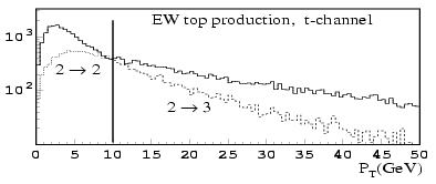
Figure 5.1: pT spectrum of the additional b in the LO 2→2 (dotted curve) and the NLO 2→3 (dashed curve) W-gluon process. The full line shows the spectrum generated by mixing the 2→2 spectrum below the 10 GeV threshold with the 2→3 spectrum above the threshold [].

5.1.2 Comparison with NLO calculation
The output of generators needs to be checked with theory in order to validate the Monte Carlo simulation. In a paper from Z.Sullivan, the events generated with Pythia and were checked against the NLO calculations of the ZTOP package []. Since both MC generators implement only the LO diagram for t-channel single top production, the pT spectrum of the additional b in the generated sample is softer than the spectrum predicted by the NLO calculation.
Using the same ZTOP results, I performed a comparison between the NLO calculations and the results. First of all, I ran ZTOP, generating the differential distributions for the t-channel. The selected set parton distribution functions was CTEQ5M and the factorization and renormalization scales were set to Q2 for light quarks and Q2+mt2 for the top quark. The final state included the top quark --- ZTOP does not simulate top decay --- and at least one reconstructed jet with pT>10 GeV, |h|<5.
The sample was composed of 20000 events generated with the CTEQ5L PDF (which is better suited for LO distributions), and with factorization and renormalization scales set to mt. Since the cross-section calculated by ZTOP is for kT jets, not particles, I ran a jet algorithm on the particle list output by +Pythia. I used a kT algorithm with cut parameter D=0.54 --- which is equivalent to a cone of R=0.4 for cone algorithms --- and with a energy threshold of 10 GeV. Then, I proceeded to identify the jets in the list: a jet was tagged as a b-jet if a b-quark from the MC truth was found inside the jet cone. The b-jet from the top decay was discarded, and the pT spectra of the additional b-jet and the light jet were compared with the ZTOP results.
To proceed with the comparison, first of all a multiplying factor was applied to all histograms, in order to obtain the same cross-section between and ZTOP:
| K= |
|
= |
|
~0.985 |
The pT and h distributions of the generated top quark are shown in Figures ?? and ??. The distributions agree with the ZTOP previsions.
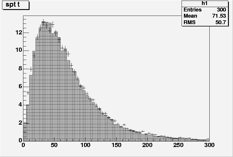
Figure 5.2: pT distribution of the top quark by NLO predictions (red) and . The histograms are normalized to the NLO cross-section.

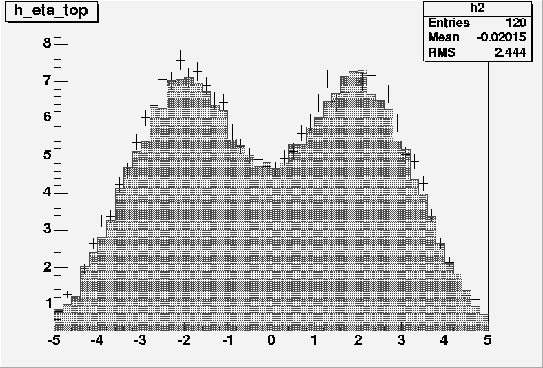
Figure 5.3: h distribution of the top quark by NLO predictions (red) and . The histograms are normalized to the NLO cross-section.

The pT spectra for light jets and b-jets are shown respectively in Figures ?? and ??. The light jet spectrum is roughly consistent with the NLO predictions, but the b-jet spectrum has an integrated cross-section which is considerably considerably lower than the NLO predictions. The cross-section for b-jets with pT>50 GeV is 26% lower than the corresponding cross-section from NLO; after applying a scaling factor to compensate for the different cross-section, the eta spectrum is compatible with the NLO predictions. Thus, the presence of an additional b-jet in the data sample is underestimated. Since the selection cuts for the t-channel sample require the presence of only one b-jet with pT>50 GeV (see Section ??), the selection efficiency from real data could be lower than from the MC sample.
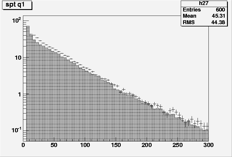
Figure 5.4: pT distribution of light jets by NLO predictions (red) and . The histograms are normalized to the NLO cross-section.

pT distribution of b-jets by NLO predictions (red) and . The histograms are normalized to the NLO cross-section.
Figure 5.5:

5.2 Parton Shower Algorithms
Pythia. Brief description of the string model
5.3 Fast simulation
5.3.1 ATLFAST
Atlfast algorithm chain:
- Cell Maker and Clu. All particles are divided in cells of granularity 0.1×0.1 for the barrel and 0.2×0.2 for the endcap. The f angle is smeared according to two parametrizations of the magnetic fields in the barrel and in the endcap. All cells with Et>1.5 GeV are selected as cluster seeds and listed in descending order. For each seed, all cells inside a cone of D R<0.4 belong to the cluster. A cluster is accepted if the total Et is higher than 10 GeV and the cells used are removed from the list; thus jet energy sharing is not implemented. Atlfast can also be instr ucted to use kT or sliding window algorithms.
- Isolator. The isolator algorithm associates each reconstructed cluster with a particle of the MC truth. The associated particle must have |h|<2.5, pt>10 GeV and with a separation D R<0.1 from the cluster baricenter. The particle is declared as isolated if the associated cluster is atleast D R>0.4 away from the closest reconstructed cluster and the transverse energy deposited in a cone D R<0.2 around the particle is lower than 10 GeV. Photons, Electron and Muons follow the same procedure. Muons have a lower pT threshold (6 GeV) and, in addition, receive a pT smearing. The smearing in the Inner Detector is given by The smearing in the Muon Spectrometer is not documented.
δ pT pT =5×10⁻⁴⊕0.012 - Jet Maker. Unidentified clusters are treated as hadron jets and smeared with the following (low-luminosity):
δ E E = 0.5 E ⊕0.03 (barrel) For high luminosity, a pile-up term of 7.5 GeV Et is added to non-empty cells. Non-isolated muons are added to jet energy too. If the total Et exceeds 15 GeV, the hadron jet is accepted.δ E E = 1.0 E ⊕0.07 (endcap) - Missing Et. The total Et of the event is computed by summing the transverse momenta of identified isolated particles, hadronic jets, non-isolated muons and unused clusters and cells. The missing Et is obtained by balancing the total Et. Thus it contains neutrinos, SUSY particles (if any) and muons outside the detector acceptance. Since by construction ATLFAST does not add pileup to empty cells, the Missing energy might be a little higher than the true value. .
- Atlfast-B. This algorithm calibrates the jet energy of b-jets, on the premise that b-jets have usually a lower energy than the originating b-quark, because of the presence of leptons (and hence neutrinos) in the decay chain. This algorithm, moreover, provides a realistic b-tagging and c-tagging efficiency, as opposed to the next to 100% efficiency of the standard ATLFAST algorithm.
5.4 Full Simulation
(Very brief, just an outline on GEANT4 and the Rome Layout)
5.5 ATHENA and the ATLAS Data Model
What do I find inside an AOD?
5.6 The Rome Data Challenge
5 Million events of various nature. Single top samples:
- 100k W-gluon fusion
- 40k+40k Associated production
- 60k s-channel
- 25k+25k W-gluon fusion with FCNC decays
- W+2jets
- W+3jets
- W+4jets
- Wbb
- tt MC@NLO
--Barison 13:47, 12 Oct 2005 (MET DST)