Difference between revisions of "Tools to scan the mSUGRA phasespace"
| (3 intermediate revisions by the same user not shown) | |||
| Line 1: | Line 1: | ||
| − | This document shows how to use two simple macros, susygen.py and susymap.py, to scan any part of the 5D mSUGRA phasespace. | + | This document shows how to use two simple macros, susygen.py and susymap.py, to scan any part of the 5D mSUGRA phasespace. These macros can only scan for information calculated by IsaSugra (mostly only the SUSY mass spectrum), as no events are generated. To automatically generate AtlFast SUSY events look at: *[[Generating_AtlFast_SUSY_Events | Generating AtlFast SUSY Events ]] |
= '''IsaSugra''' = | = '''IsaSugra''' = | ||
| Line 7: | Line 7: | ||
At Nikhef the most resent IsaSugra release (7.75) is installed at /project/atlas/users/nicoleru/Store/isajet/isasugra.x | At Nikhef the most resent IsaSugra release (7.75) is installed at /project/atlas/users/nicoleru/Store/isajet/isasugra.x | ||
| + | |||
| + | When studying a susypoint with |A0|>0, keep in mind that some theoretical papers use a deffinition of A0 that differs by a minus sign from the one used by programs such as IsaSugra. | ||
= '''Scanning the mSUGRA phasespace''' = | = '''Scanning the mSUGRA phasespace''' = | ||
| Line 49: | Line 51: | ||
= '''How to use''' = | = '''How to use''' = | ||
| − | Both macros (susygen.py and susymap.py) should be easy to use. Just copy them to | + | Both macros (susygen.py and susymap.py) should be easy to use. Just copy them to your own directory. They are both located at: /project/atlas/users/nicoleru/Store/. |
As long as you are only interested in the information currently optained by susygen.py, you only need to change susymap.py to form your own 5D susy grid. If you need additional information, the mass of one of the susy particles for example, it will take slightly more work, as you need to know exactly where that information is printed in the IsaSugra output files. If you have any problems getting this additional information, just ask me (Nicole). | As long as you are only interested in the information currently optained by susygen.py, you only need to change susymap.py to form your own 5D susy grid. If you need additional information, the mass of one of the susy particles for example, it will take slightly more work, as you need to know exactly where that information is printed in the IsaSugra output files. If you have any problems getting this additional information, just ask me (Nicole). | ||
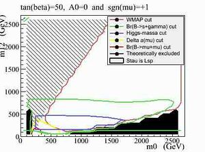
Making the plots is more difficult as I don't have one root file that, when you feed it a susymap file, simply gives you a plot similar to figure 1. I will work on that. In the mean time, the root file used to make figure 1 should easily be convertible to other grids. | Making the plots is more difficult as I don't have one root file that, when you feed it a susymap file, simply gives you a plot similar to figure 1. I will work on that. In the mean time, the root file used to make figure 1 should easily be convertible to other grids. | ||
Latest revision as of 14:20, 17 April 2008
This document shows how to use two simple macros, susygen.py and susymap.py, to scan any part of the 5D mSUGRA phasespace. These macros can only scan for information calculated by IsaSugra (mostly only the SUSY mass spectrum), as no events are generated. To automatically generate AtlFast SUSY events look at: * Generating AtlFast SUSY Events
IsaSugra
IsaSugra is a subprogram of IsaJet that calculates the mass-spectrum and decay-channels for a number of SUSY models, including mSUGRA. As input parameters, for mSUGRA, it requires the mSUGRA coordinate and the top mass. The output can take different forms of which two are important here. The first is a text file including all SUSY and Higgs masses and decay channels. This file can be used directly in Jimmy to produce events. The second is a more easily read text file also including all masses and decay channels, but in addition also containing some SM values that may be affected by SUSY, such as , , and which is the cold dark matter relic density this SUSY point would produce.
If the susy point under consideration is theoretically not allowed (for example because at this point no electroweak symmetry breaking is possible), IsaSugra will give an error, indicating the reason why the susy point was rejected.
At Nikhef the most resent IsaSugra release (7.75) is installed at /project/atlas/users/nicoleru/Store/isajet/isasugra.x
When studying a susypoint with |A0|>0, keep in mind that some theoretical papers use a deffinition of A0 that differs by a minus sign from the one used by programs such as IsaSugra.
Scanning the mSUGRA phasespace
The macro susygen.py runs IsaSugra for a certain susypoint and checks if it is theoretically valid. If it is valid it retrieves certain values from the output files. The information gathered by susygen.py is printed to a text file. At present the following values are written (in this order on one line):
M0, M12, A0, tan(beta), sgn(mu), theory, lightest neutralino mass, lightest Higgs-boson mass, the LSP, BR(b->s+gamma), omega*h^2, Br(Bs->mu+mu) and delta a(mu).
The values are given in GeV (when applicable). The theory value is either 0 (ok) or 1 (not valid) and if 1 no further information is included. The LSP is indicated using the particle numbering of Herwig (lightest neutralino = 450, stau = 429).
susymap.py is a simple program that defines a grid (with evenly separated point in any variable) in the 5D mSUGRA phasespace and starts the text file in which all information will be printed (it also adds a line indicating which variables will be printed). susymap.py will call susygen.py for each point on the grid. The result of this program is a file indicating all relevant information about a large number of susypoints.
Examples of results
As an example of the use of these macros I have run them for a 2D grid, with tan(beta)=50, A0=0 and sgn(mu)=+1 fixed. Both m0 and m12 are varied in 25 steps from 100 to 2500 (so basically 625 point). On stoomboot (submitted in 1 job) this took approximately 3 hours. The output file is located at /project/atlas/users/nicoleru/Store/map_A0_0_tan_50_si_1.txt. The first few lines of that file are the following:
   m0   m12    A0   tan  sign  EWSB   neutalino   Higgsmass  LSP  BR(b->s+gamma)      omega*h^2    Br(Bs->mu+mu)    dela a(mu)
  100   100     0    50     1     1
  100   200     0    50     1     1
  100   300     0    50     1     1
  100   400     0    50     1     1
  100   500     0    50     1     1
  100   600     0    50     1     1
  100   700     0    50     1     0  292.791500  116.384600  429    2.747800e-04   1.000000e+04    1.181600e-08   2.434000e-09
  100   800     0    50     1     0  336.540300  116.977000  429    2.909800e-04   1.000000e+04    9.644800e-09   1.876200e-09
  100   900     0    50     1     0  380.830800  117.482900  429    3.016500e-04   1.000000e+04    8.222600e-09   1.488700e-09
  100  1000     0    50     1     0  424.931700  117.990400  429    3.092800e-04   1.000000e+04    7.275100e-09   1.209400e-09
  100  1100     0    50     1     0  469.779800  118.380700  429    3.149100e-04   1.000000e+04    6.617900e-09   1.001000e-09
  100  1200     0    50     1     0  514.302500  118.781100  429    3.194900e-04   1.000000e+04    6.133900e-09   8.418700e-10
  100  1300     0    50     1     0  559.054500  119.079700  429    3.213500e-04   1.000000e+04    5.769000e-09   7.175600e-10
Using a root file to put all this information in a plot leads to figure 1. (/project/atlas/users/nicoleru/Store/rootfilefigure1.C)
Of course this program can also be used to plot a A0-tan(beta) plain, or to see how certain variables change close to the point you are studying.
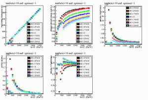
As an example of other possible use of this program, I have extended the grid used in the first example to include different values of A0 (and changed tan(beta) to 10), namely A0={-3,-2,-1,0,1,2,3}*m12. Due to WMAP information, most of the m0-m12 plane is excluded. Only two very thin lines remain, one that borders the LSP=stau area, and one line at very low m12. Due to this, we can basically reduce the 5D mSUGRA phasespace to 4D, by relating m0 to m12. Using another root file, it is possible to plot the (lightest) Higgs-mass, or Br(B->s+gamma) or any other variable, as function of m12, for fixed A0, tan(beta) and sgn(mu). (/project/atlas/users/nicoleru/Store/rootfilefigure2.C)
How to use
Both macros (susygen.py and susymap.py) should be easy to use. Just copy them to your own directory. They are both located at: /project/atlas/users/nicoleru/Store/.
As long as you are only interested in the information currently optained by susygen.py, you only need to change susymap.py to form your own 5D susy grid. If you need additional information, the mass of one of the susy particles for example, it will take slightly more work, as you need to know exactly where that information is printed in the IsaSugra output files. If you have any problems getting this additional information, just ask me (Nicole).
Making the plots is more difficult as I don't have one root file that, when you feed it a susymap file, simply gives you a plot similar to figure 1. I will work on that. In the mean time, the root file used to make figure 1 should easily be convertible to other grids.


