Difference between revisions of "Chapter VI"
| Line 163: | Line 163: | ||
Select the top with the highest pt. Works well, but the physics of it escapes me.<BR> | Select the top with the highest pt. Works well, but the physics of it escapes me.<BR> | ||
<BR> | <BR> | ||
| + | |||
| + | [[Image:Bkg+sig.gif]] | ||
| + | |||
| + | [[Image:Bkg+sig04.gif]] | ||
| + | |||
<!--TOC section Systematics--> | <!--TOC section Systematics--> | ||
Revision as of 16:01, 12 October 2005
--Barison 14:38, 12 Oct 2005 (MET DST)
Chapter 6 Analysis
- single top channels are little affected by combinatorics
- however ttbar and wjj backgrounds are dominant
- need to find good trade-off between selection efficiency and background rejection
6.1 AOD Definitions
Insert work on: electron selection, bjet tagging
6.1.1 Electrons
In the AOD data file, two types of electron candidates are present, reconstructed with different algorithms:
- the softe algorithm, which is optimised to reconstruct electron candidates with pT< 10 GeV;
- the egamma algorithm, which reconstructs hard electrons.
Since electrons from single top decays are highly energetic, in my analysis I will consider egamma electrons only. There are also two methods to discriminate between electrons and pions/photons in the candidate list:
- the isEM flag, which is a 16-bit word where each bit represents the result of a discriminating algorithm. The candidate is an electron if isEM = 0.
- the "weight" which assigns to the candidate a probability of being an electron or a pion/photon. The candidate is an electron if
We We+Wp >0.6
Finally, the single top analysis requires isolated electrons. To define isolation, the total transverse energy deposed in a 0.2 cone around the electron needs to be lower than 10 GeV. This definition matches the isolation cut defined in ATLFAST (see Section ??).
I performed an analysis to investigate which one of the two discriminating methods gives the best results for identifying electrons. First of all I searched for the true electron from the W decay in the MC truth. Then, I ordered the reconstructed electrons by descending pT. I obtained two lists, one for each selection method. From each list I considered only the highest pT electron. Then I analysed the pT spectra, the efficiency of the two methods, and the angular resolution w.r.t. the MC truth.
pT Spectrum

The plot shows the Pt spectrum of the MC electrons (black), the isEM electrons (red) and the Likelihhod electrons (blue). Nothing wrong in the spectrum, but it is obvious that the Likelihood choice gives higher efficiency,and a few fakes.
Efficiency
By defining efficiency as the probability of finding exatcly one electron above a 20 GeV threshold, efficiency for isEM is 70.7
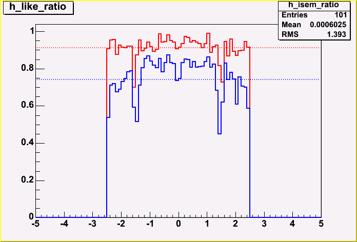
Figure 6.1: Efficiency w.r.t. Pseudorapidity for the two choices. The cracks in the intermediate region are clearly visible.

pT Resolution
Ratio between the Pt of reconstructed electron and the true electron. Percentage of events with ratio inside (20%, 40%, 60%) for isEM:
96.1% -- 98.2% -- 99.1%
Percentage of events with ratio inside (20%, 40%, 60%) for Likelihood:
91.6% -- 94.7% -- 96.2%
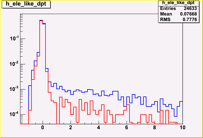
Figure 6.2:

Angular Resolution
I plot the angular distance between the true electron and the highest Pt electron candidate.
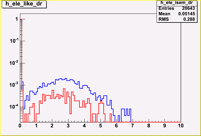
Figure 6.3:

Fake Rate
If there are no hard electrons in the MC truth, I count the reconstructed electrons as fakes. The ratio of fakes that go over a 20 GeV threshold is 0.3% for isEM and 1.6% for Likelihood.
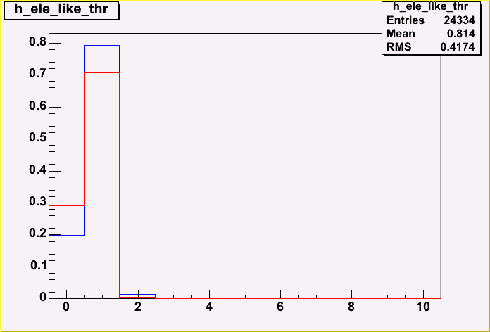
Figure 6.4:

Charge
In this plot I compare the charge of the MC electron with the charge of the reconstructed electron with the highest pt. The bin labelled "1" identifies a correct cha rge match, while "-1" identifies a charge mismatch. The mismatch rate for isEM is 0.8% while for Likelihood is 3.5%
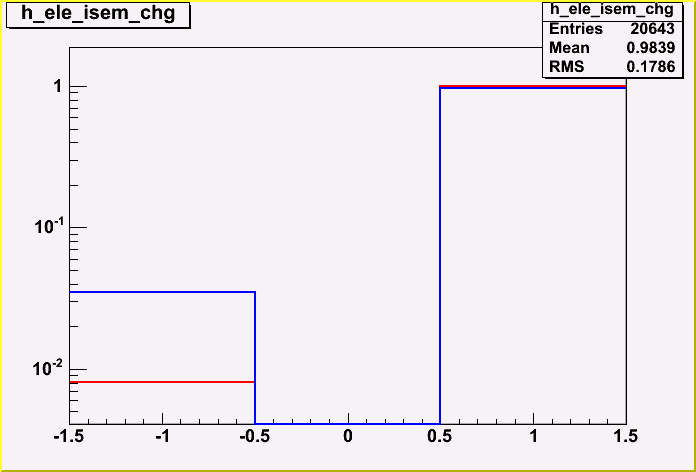
Figure 6.5:

Conclusions
Overall, isEM offers a slightly better performance in term of angular resolution, momentum resolution and charge identification. However, this is offset by the high efficiency of the Likelihood.
If precision measurements are necessary, the isEM method is preferrable (though lets not forget it is currently buggy, and its performance could improve in future SW releases).
If the analysis is performed on a small sample, and reconstruction efficiency has to be maximized, the Likelihood method is a better choice.
6.2 Selection cuts
Cut efficiency studies in the past have been performed with old montecarlo generator.
As first check, the efficiency is now lower (50%). Need a better study of cut efficiecies.
- isolated lepton cut: trigger efficiency, cut efficiency
- b-tagging: why do we use single instead of double b-tag (collinear b)
- forward light jet: discriminant against Wjj backgrounds
- no cut on missing Et. Need to insert one?
Here put a graph of the selection cuts with the efficiencies.
- Isolated lepton distributions
- Jet distribution
- Total invariant mass
- Other?
6.3 Kinematic fit to the W mass
- W mass measured with good resolution
- W mass can be used for calibration purposes (ttbar, usually)
- Quadratic function: two results. Good need handle on missing Et
6.4 Combinatorics and Top selection
There are almost no combinatorics, however there is a double ambiguity. A few methods to solve it:
6.4.1 Target mass
Retain the solution with mass closest to 175. It biases the event.
6.4.2 Reverse boost
Boost all the decay particles back to the top frame and select the couple close to the back-to-back configuration. It does not work very well (jet scale might be a problem).
6.4.3 Highest Pt
Select the top with the highest pt. Works well, but the physics of it escapes me.
6.5 Systematics
6.5.1 Minimum bias
Minimum bias events are events where the colliding protons undergo a soft elastic collisions or a soft parton collision (diffractive events). Occasionally, a soft parton collision might "fluctuate" to result in an event with high enough pT to be measured by the detector.
Underlying events are defined as the sum of all types of events (beam remnants, ISR, secondary parton collisions) which happen at the same time of hard inelastic parton scattering. In the first approssimation, underlying events and minimum bias events are assumed to be governed by the same physical model. However, there can be significant differences, since color interactions between the hard scattering and the underlying events might occur, modifying the spectra of the two classes of events.
At the detector level, underlying events generate extra tracks in the detector and deposit energy in the calorimeter, thus degrading the measurement of the hard scattering. Several studies have been performed to evaluate the effect of underlying events by modelling minimum bias in Montecarlo generators and using the same model to generate underlying events.
In PYTHIA, the model of minimum bias is the following: the number of underlying events is given by the ration between the cross section for "hard" minimum bias events divided by the cross-section of total, inelastic non-diffractive soft events: shard(p^ min)/snd(s). While p^ min in principle should be zero, in practise a cut off must be included to prevent the aforementioned ratio to diverge. The minimum momentum applicable is calculated at run-time by PYHTIA with the following formula:
| p^ min(s)=p82 |
/ |
|
\ |
|
, |
where the parameters pi are defined in pythia by PARP(I). The physical meaning of this formula is that when the exchanged momentum between the scattering parton is low, the exchanged gluon cannot resolve the individual colour of the partons, reducing the coupling constant. This screening effect limits the cross-section at low momenta.
The effect of the impact parameter on the minimum bias collision is parametrized by a double-gaussian parton density:
| r(r)μ |
|
exp |
/ |
- |
|
\ |
+ |
|
exp |
/ |
- |
|
\ |
, |
which describes a parton model when a fraction b of the hadronic matter is contained inside a "core" the radius of which is a2/a1 of the proton radius. This model correctly describes the multiplicity of minimum bias events: harder collisions result in smaller impact parameter, which probes high density regions where minimum bias events are more likely to happen.
Minum bias was studied at CDF by Rick Field et al. to obtain a PYTHIA tuning capable do describe data. The method utilised at CDF is the following: minimum bias data is generated by PYTHIA by selecting MSEL=1 (QCD high- and low-pt events). For each event, jets are reconstructed with a cone of radius 0.7; the phi space is divided into four regions, using the jet with the highest pt in the event as a reference axis. Two of the zones are labelled as "transverse", and cover a region from 60 to 120 away from the jet axis. All charged particles included in these two regions are examined, event by event: the scalar pt sum of particles surviving the cut |h|<1, pT>0.5 GeV is computed, and plotted against the pt of the leading jet. A similar technique can be used by examining jets instead of individual particle, but CDF used charged tracks because of the better resolution of the tracker w.r.t. the calorimeter.
If we separate the two transverse zones in a region of low energy deposition and a region of high energy deposition and we plot separately the scalar pt sum, we obtain two separate diagrams, where the amount of high energy deposition is correlated with the "hard" fraction of minimum bias, while the low energy plot is correlatedwith the "soft" and collinear scatterings. The PYTHIA parameters were tuned to make these two plots reproduce the same plot drawn for CDF minimum bias data.
The parametrisation obtained by Field is the following:
- PARP(82)=2.0 regularization scale of the minimum pt in the hard scattering (D=2.1);
- PARP(83)=0.5 fraction of hadronic matter inside the "core" (D=0.5);
- PARP(84)=0.4 ratio between the "core" radius and the proton radius (D=0.2);
- PARP(85)=0.9 probability of having an extra interaction giving two gluons (D=0.33);
- PARP(86)=0.95 probabilty of having an extra interaction giving two gluons or a closed gluon loop (D=0.66);
- PARP(89)=1800 regularization energy of the minimum pt --- 1.8 TeV (D=1000.);
- PARP(90)=0.25 exponent of the regularization function (D=0.16);
- PARP(67)=4.0 maximum virtuality (4× Q2) for spacelike parton showers (D=1.);
The main effect of the above tuning is to increase the core size, thus reducing the parton density and thus decrease the multiplicity, and to increase initial state showers. No plot this time, I screwed up badly.
The parametrization used at DC2, instead, is very simple:
- MSTJ(11)=3 fragmentation scheme: use Peterson fragmentation function for b- and c-quarks;
f(z)= 1 z /
\
|
|
1- 1 z - (-c) 1-z \
/
|
|
2
- MSTJ(22)=2 decay cutoff: decay particles only if ct>10 mm;
- PARJ(54)=-0.07 c factor in the Peterson function for c-quarks (D=-0.05);
- PARJ(55)=-0.006 c factor in the Peterson function for b-quarks (D=-0.005);
- PARP(82)=1.8 regularization scale of the minimum pt in the hard scattering (D=2.1);
- PARP(84)=0.5 ratio between the "core" radius and the proton radius (D=0.2);
UPDATE: the Field parametrization is now default in PYTHIA. DOH!
6.5.2 Multiple interactions
Using the Pileup sample instead of the normal one.
6.5.3 Missing Et
6.5.4 Jet energy scale